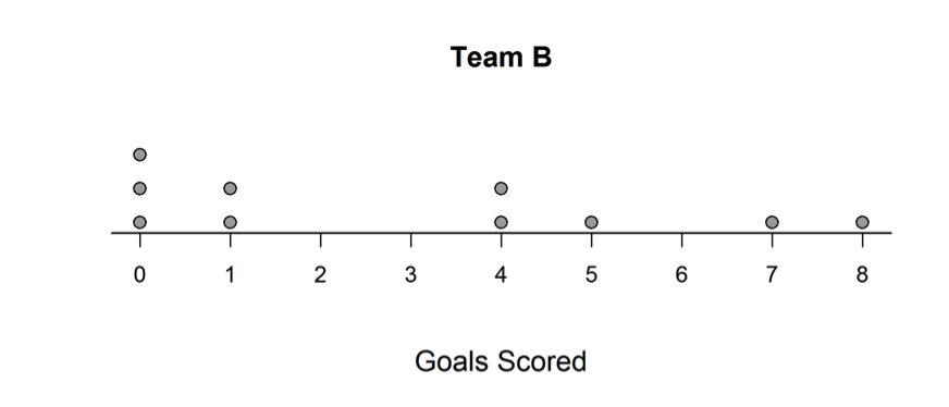
Two soccer teams will be meeting in the city championship game. Each team played 10 games and averaged 3 goals scored per game for the season. The two dotplots below show the number of goals scored by each team per game for the season.
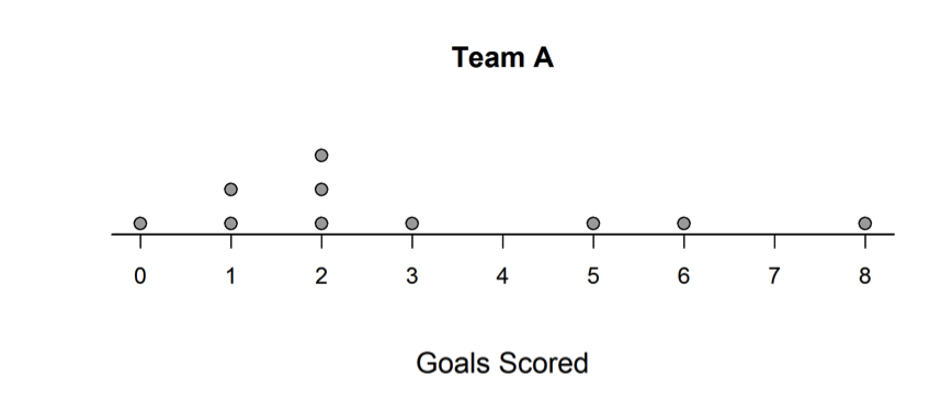
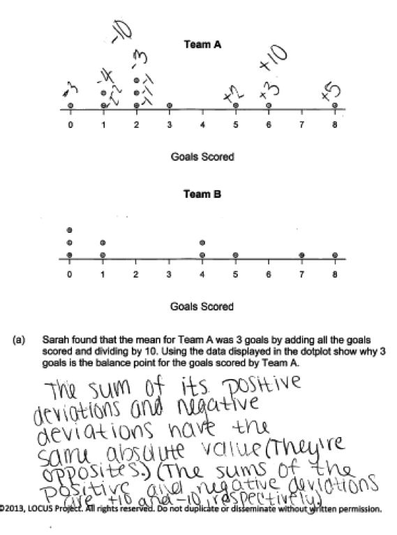
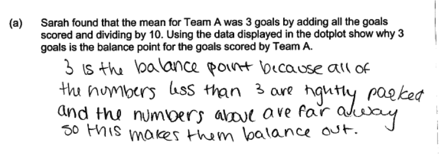
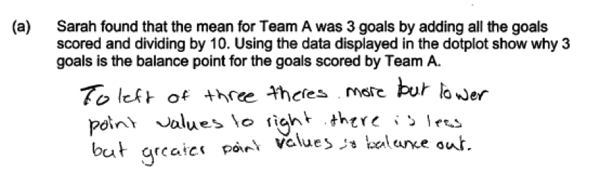
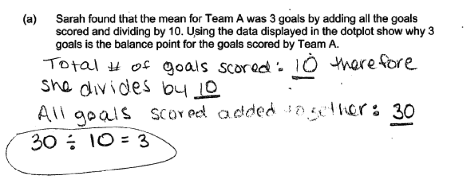
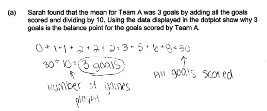
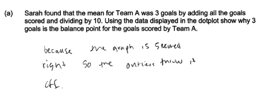
 (a) Sarah found that the mean for Team A was 3 goals by adding all the goals scored and dividing by 10. Using the data displayed in the dotplot show why 3 goals is the balance point for the goals scored by Team A.
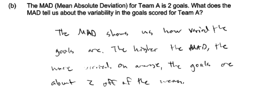
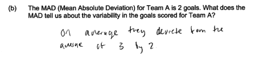
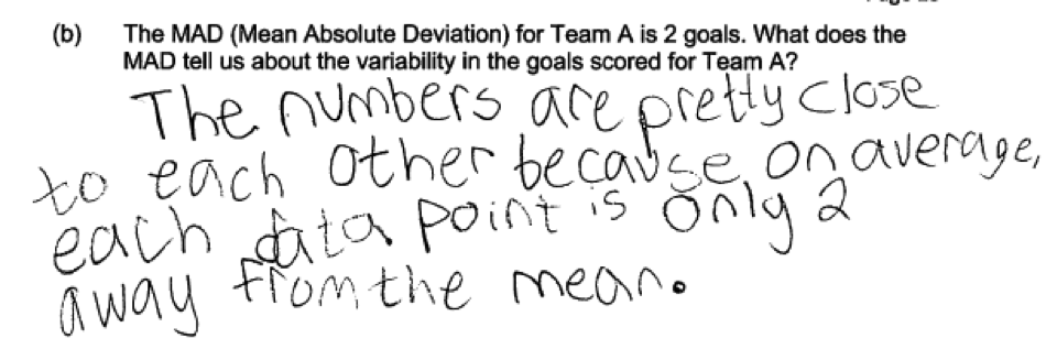
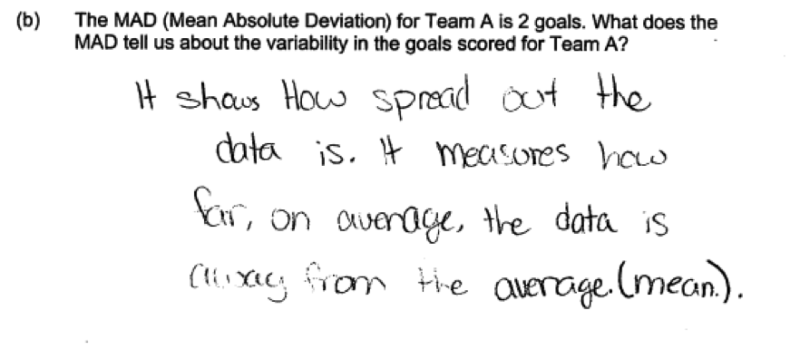
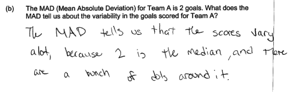
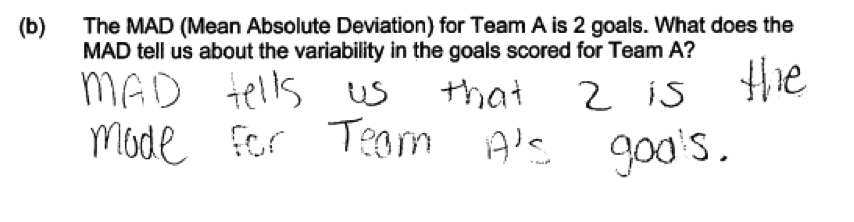
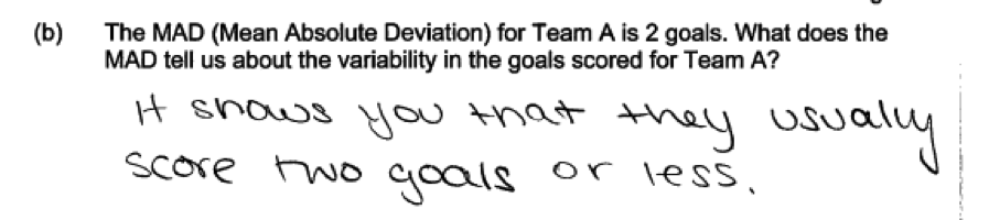
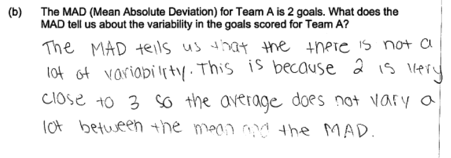
(b) The MAD (Mean Absolute Deviation) for Team A is 2 goals. What does the MAD tell us about the variability in the goals scored for Team A?
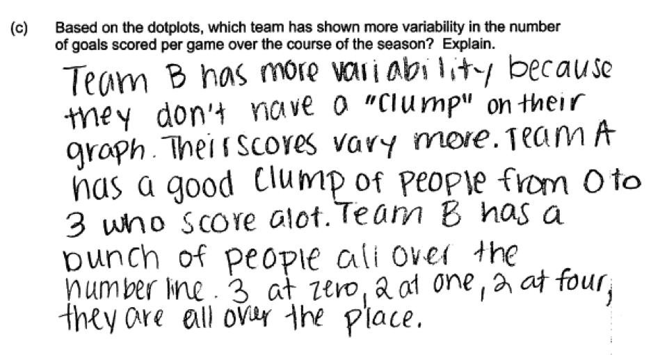
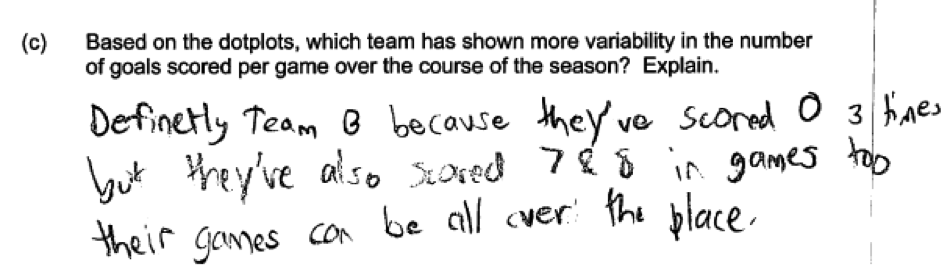
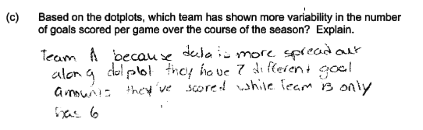
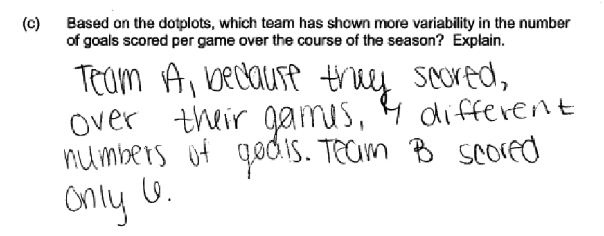
(c) Based on the dotplots, which team has shown more variability in the number of goals scored per game over the course of the season? Explain.
Overview of the question
This question is designed to assess the student’s ability to:
1. Understand the mean as the balance point of a data distribution.(part (a))
2. Interpret the mean absolute deviation (MAD) in context. (part (b))
3. Compare the variability in two data distributions given dot plots of the two distributions. (part (c)).
Standards
6.SP.5c: Summarize numerical data sets in relation to their context, such as by: Giving quantitative measures of center (median and/or mean) and variability (interquartile range and/or mean absolute deviation), as well as describing any overall pattern and any striking deviations from the overall pattern with reference to the context in which the data were gathered.
7.SP.4: Use measures of center and measures of variability for numerical data from random samples to draw informal comparative inferences about two populations.
Ideal response and scoring
Part (a):
Part (a) asks students to explain how the given mean of 3 represents the balance point for the distribution of goals scored for Team A. An ideal response to part (a) conveys an understanding of the mean as a balance point by appealing to either deviations from the mean or distances from the mean. Using deviations, an ideal response would indicate that the mean balances positive and negative deviations and that the sum of the deviations for the mean is equal to 0. A response based on distances from the mean would indicate that the mean balances the total of distances from the mean for points below the mean and the total of distances from the mean for points above the mean. Students might convey this understanding numerically or visually by showing distances marked on the given dot plot.
Part (b):
In part (a), students are given the value of the MAD for Team A and asked what this value tells them about variability in the data set. An ideal response to part (b) includes a correct interpretation of the MAD as the average distance from the mean for values in the data set. To be considered essentially correct for part (b), the interpretation of the MAD must also be in context. A response that provides a correct interpretation that is generic and not in context is considered to be partially correct.
Part (c):
An ideal response to part (c) correctly assesses variability in the given dot plots and selects Team B as the team with the greater variability. To be considered essentially correct for part (c), the response must also include a correct justification for the choice of Team B. Responses that made a choice between Team A and Team B, but which failed to provide any justification for the choice are considered to be incorrect for part (c).
Sample responses indicating solid understanding
The following student response shows a good understanding of the mean as the balance point of a data distribution. The student has correctly calculated the deviations from the mean (show on the dot plot for Team A) and provided an explanation that the mean is the point for which the sum of the positive deviations and the sum of the negative deviations are balanced. This response was scored essentially correct for part (a).
 In part (b), essentially correct responses give a correct interpretation of the MAD in context. The following student response was scored as essentially correct for part (b). It includes a correct interpretation of the value of the MAD (“on average, the goals are about 2 off the mean”) and the interpretation is in context.
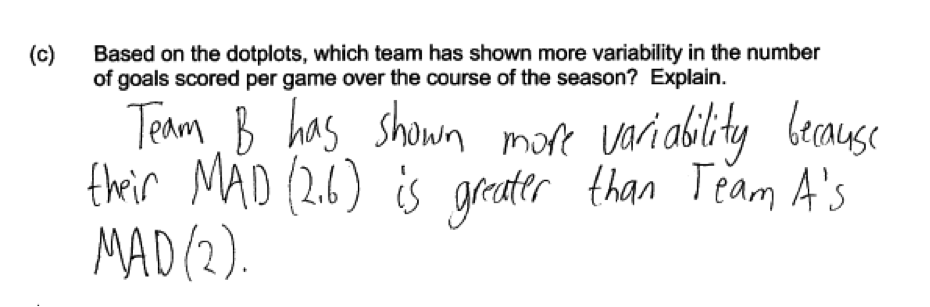
 In part (c), there are several ways that a student might correctly justify the choice of Team B as the data set with the greater variability. Because part (b) gave the MAD for the Team A data set, some students chose to compute the MAD as a measure of variability for the Team B data set and then use the MAD to select the data set with greater variability. This approach is illustrated in the following student response, which was scored as essentially correct for part (c).
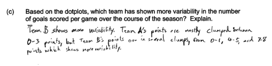
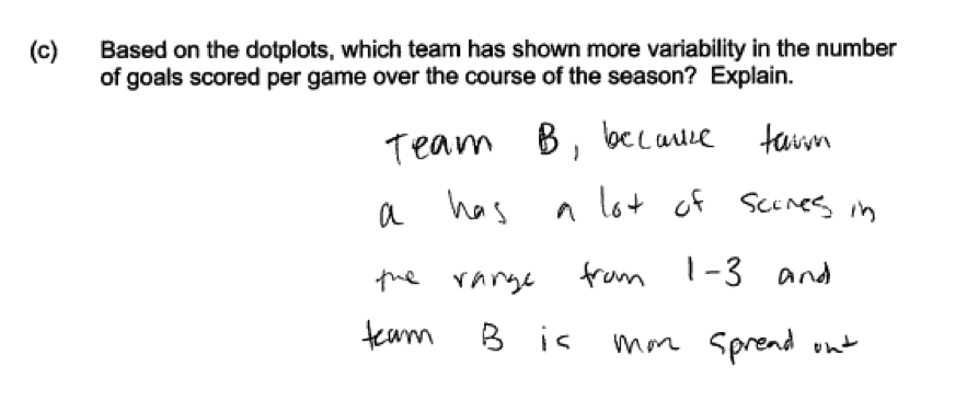
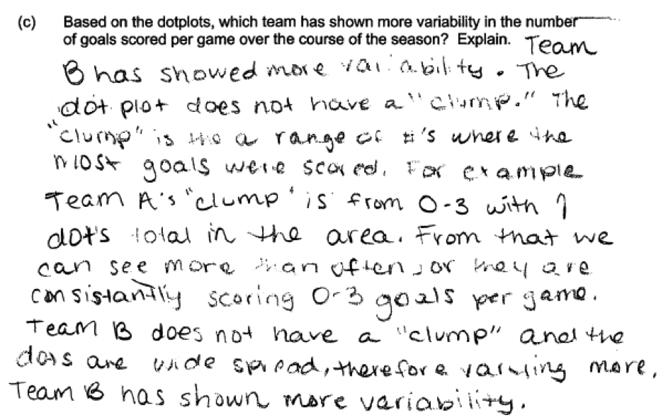
 It is also possible to assess the variability visually using the dot plots and to base a justification on the way that the data values are distributed along the number line. The following four student responses illustrate this approach and were all scored as essentially correct for part (c).
Common misunderstandings
Part (a) Understand the mean as the balance point of a data distribution.
Students struggled with part (a) and not many student responses demonstrated an understanding of the mean as the balance point of a data distribution. Of those students who did try to get at the idea of the mean as a balance point, many provided only a weak explanation that did not directly appeal to deviations from the mean or distances from the mean. The following two student responses are responses that illustrate such a description.
 Many students did not really address the idea of balance point at all and just used the data presented in the dot plot to verify that the mean was equal to 3, as illustrated in the two responses that follow.
 Another common mistake was to focus on the effect of outliers on the sample mean rather than on the idea of mean as a balance point of a data distribution. The student response below is typical of responses that made this error.
Part (b) Interpret the mean absolute deviation (MAD) in context
There were two common errors in answering part (b). Some students did not realize that interpretations should always be in context. This resulted in responses that were scored as only partially correct, even though they may have included a correct generic interpretation of the MAD. Each of the following three responses were scored as partially correct because of this error, but could have been scored essentially correct if they had been in context.
 Many students indicated a lack of understanding of the MAD as a measure of variability and provided incorrect interpretations of the MAD in their responses. Each of the four student responses below illustrates a different incorrect interpretation of the MAD. These incorrect interpretations indicate that students did not have an idea of what the MAD measures and that they may not have worked with the MAD as a measure of variability. This may improve with the inclusion of the MAD as part of the 6th grade curriculum under the Common Core.
Part (c) Compare the variability in two data distributions given dot plots of the two distributions
In part (c) students needed to assess the variability in two data sets that have been displayed in dot plots, indicate which data set had the greater variability, and justify their choice. There were two common errors that students made in part (c) that resulted in scores of partially correct or incorrect for this part.
One common error was made by students who correctly chose Team B as the data set with the greater variability, but provided a weak explanation for the choice. The student response below is a response that was scored as only partially correct because the explanation was considered weak.
 The second common student error was to select Team A as the data set that exhibited the most variability. This error could result in a score of partially correct or incorrect, depending on the explanation provided. The student response below is an example of one that received a score of incorrect for part (c). The student has selected Team A and the justification for the choice is incorrect. The range is equal to 8 for both data sets, and the statement about the ratio of number of goals addresses center rather than spread in the data sets.
 There was one way that a student could justify a choice of Team A and receive a score of partially correct for part (c). In each of the two student responses that follow, the student supports the choice of Team A by appealing to the fact that Team A scored more different numbers of goals (0,1,2,3,5,6,8 for Team A and 0,1,4,5,7,8 for Team B). Responses that were based on this justification for selecting Team A were scored as partially correct for part (c).
Resources
More information about the topics assessed in this question can be found in the following resources.
Free Resources
Classroom and Assessment Tasks
Illustrative Mathematics has peer reviewed tasks that are indexed by Common Core Standard.
A task that includes the comparison of the variability in two data distributions is
This links to another task that includes interpreting the MAD and comparing variability in two data distributions.
Guidelines for Assessment and Instruction in Statistics Education (GAISE)
Published by the American Statistical Association and available online, this document contains a nice discussion of the mean as a balance point of a data distribution in the section titled “A Measure of Location—The Mean as a Balance Point” (pages 41 – 43). It also includes a section that develops the mean absolute deviation (MAD) as a measure of variability (“A Measure of Spread—The Mean Absolute Deviation”, page 44).
Resources from the American Statistical Association
Bridging the Gap Between Common Core State Standards and Teaching Statistics is a collection of investigations suitable for classroom use. This book contains an investigation that introduces the mean absolute deviation (MAD) and includes a discussion of how the value of the MAD is interpreted (“How Long Are Our Shoes?”, pages 98 – 110).
Resources from the National Council of Teachers of Mathematics
The NCTM publication Developing Essential Understanding of Statistics in Grades 6 – 8 includes a discussion of measuring the amount of variability in a distribution (pages 24 – 28).