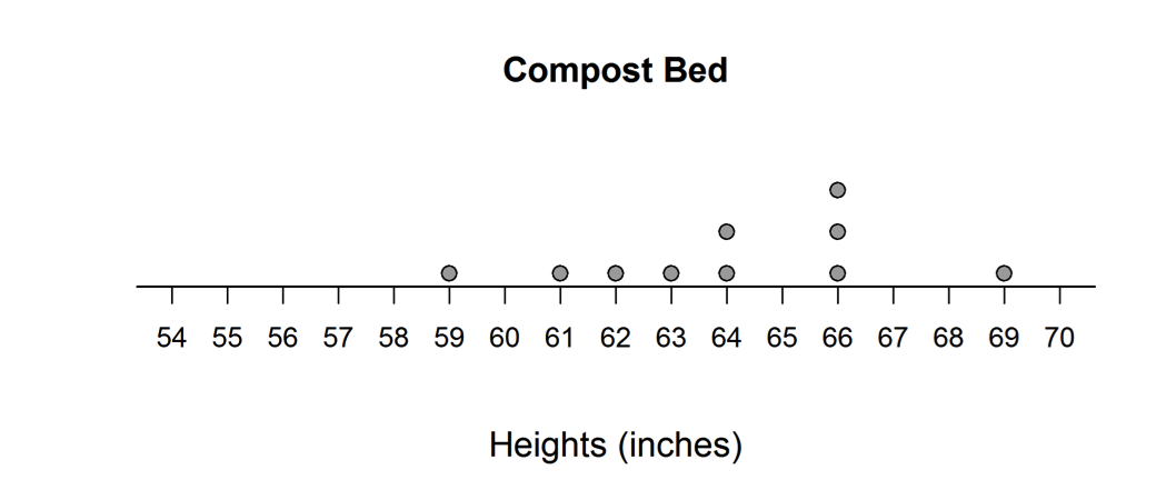
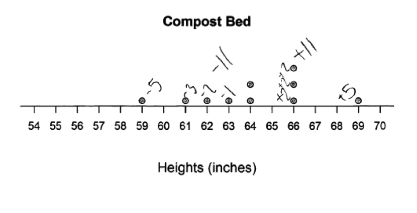
Middle school science students wanted to compare the effect of compost on the plant height of their favorite flower, the dahlia. They had two similar planting areas (called beds) except that one was treated with compost and the other was not. In designing their experiment, they tried to control as many variables as they could think of so that any observed height difference in the plants would be due to the no-compost/compost treatments and not something else. Of 20 similar dahlia plants of the same variety and height, they randomly assigned 10 of them to plant in the no-compost bed and 10 in the compost bed. The heights (inches) of the plants after eight weeks are displayed in the dotplots below.
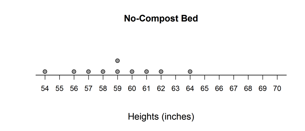
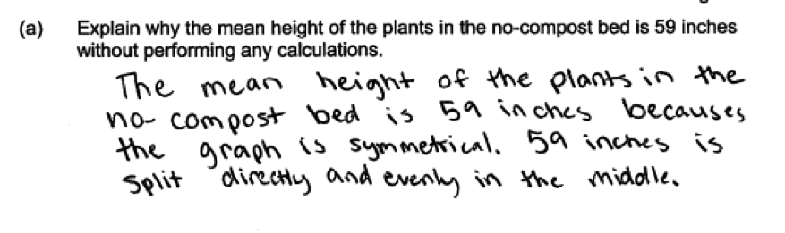
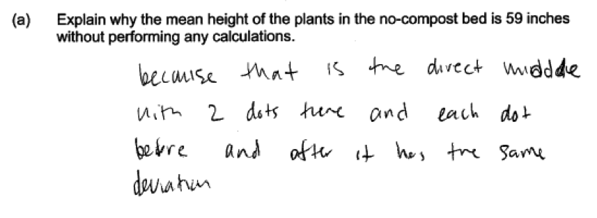
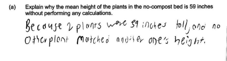
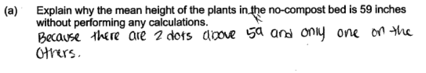
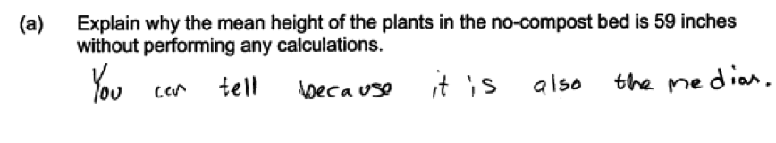
 (a) Explain why the mean height of the plants in the no-compost bed is 59 inches without performing any calculations.
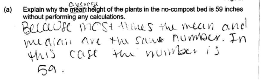
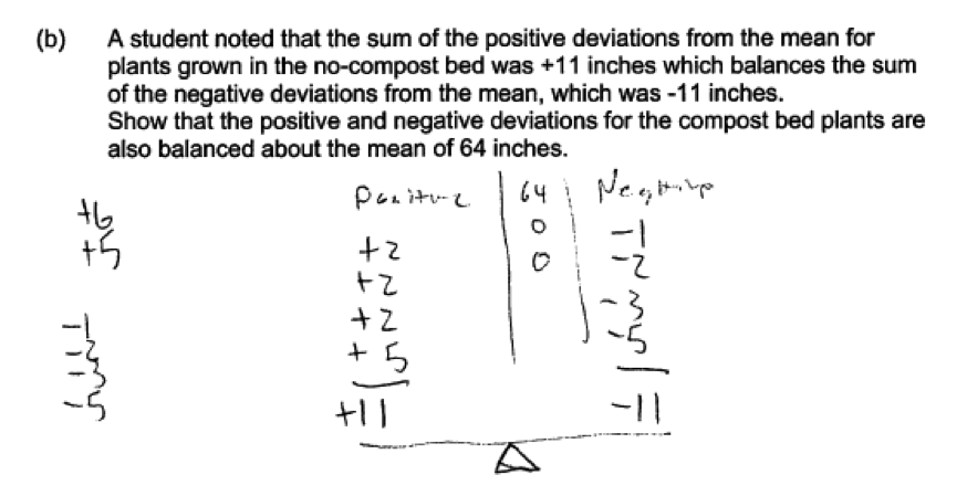
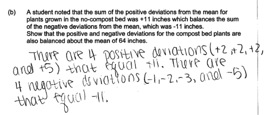
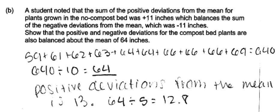
(b) A student noted that the sum of the positive deviations from the mean for plants grown in the no-compost bed was +11 inches which balances the sum of the negative deviations from the mean, which was -11 inches. Show that the positive and negative deviations for the compost bed plants are also balanced about the mean of 64 inches.
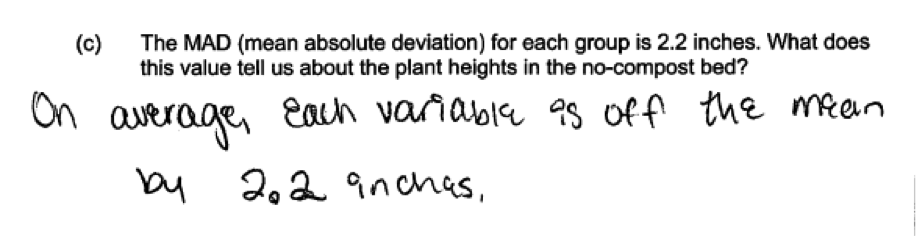
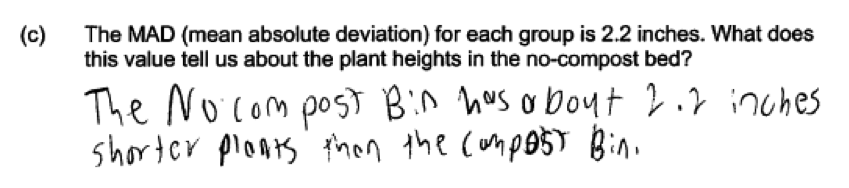
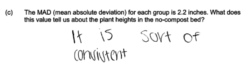
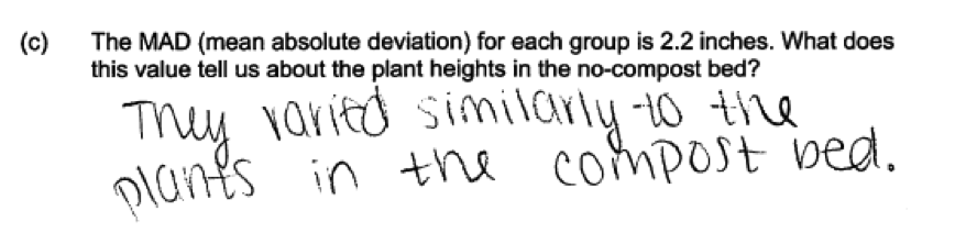
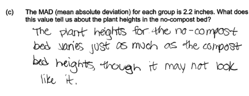
(c) The MAD (mean absolute deviation) for each group is 2.2 inches. What does this value tell us about the plant heights in the no-compost bed?
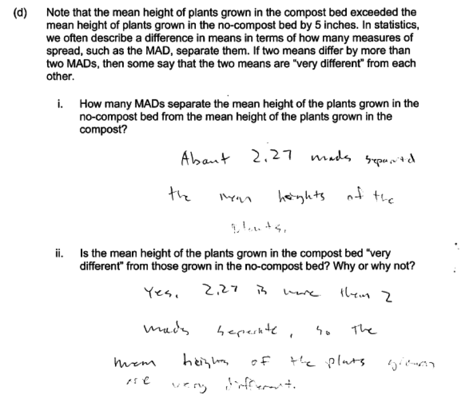
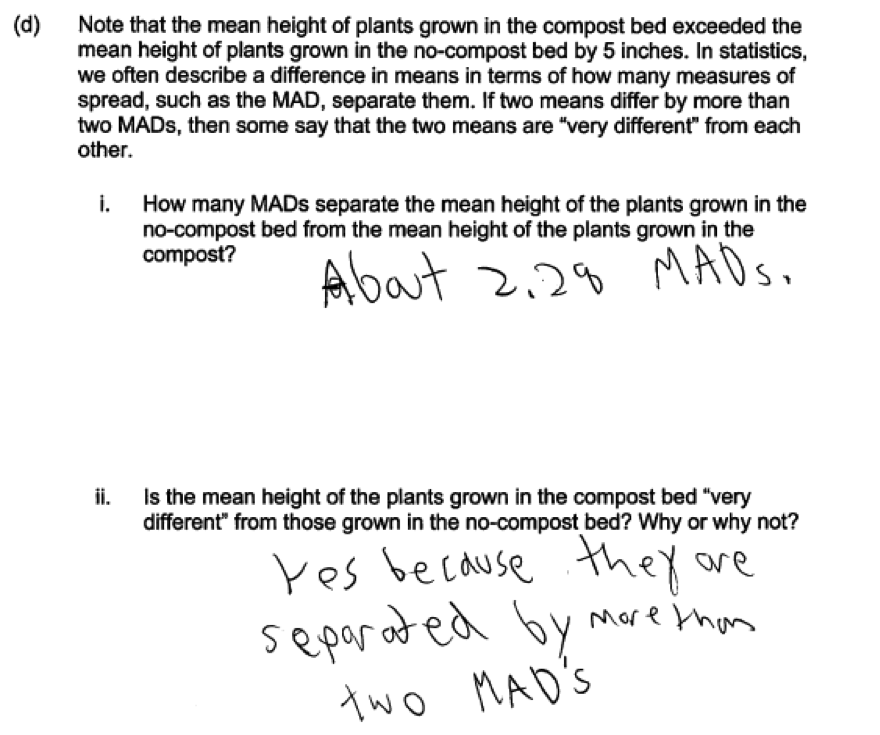
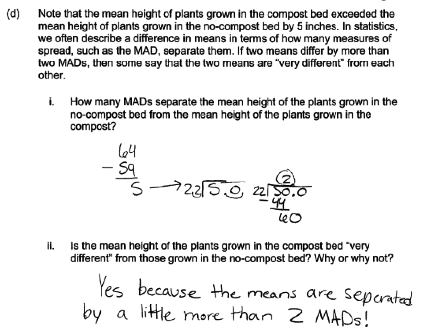
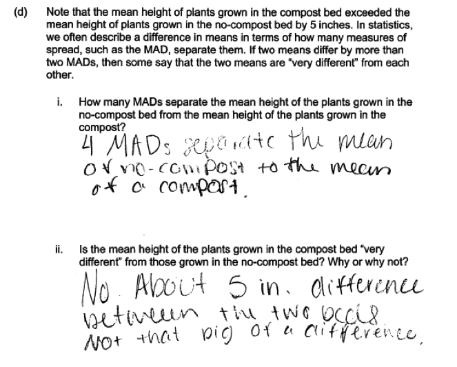
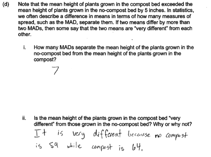
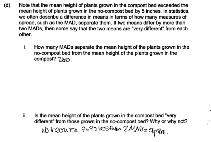
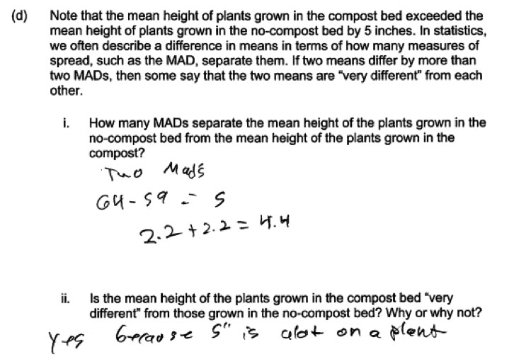
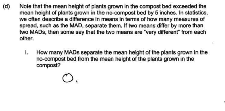
(d) Note that the mean height of plants grown in the compost bed exceeded the mean height of plants grown in the no-compost bed by 5 inches. In statistics, we often describe a difference in means in terms of how many measures of spread, such as the MAD, separate them. If two means differ by more than two MADs, then some say that the two means are “very different” from each other.
(i) How many MADs separate the mean height of the plants grown in the no-compost bed from the mean height of the plants grown in the compost?
(ii) Is the mean height of the plants grown in the compost bed “very different” from those grown in the no-compost bed? Why or why not?
Overview of the question
This question is designed to assess the student’s ability to:
1. Understand the mean as a balance point (part (a)).
2. Verify that the mean is the point for which the sum of the positive deviations and the sum of the negative deviations are equal (part (b)).
3. Interpret the mean absolute deviation (MAD) in context (part (c)).
4. Informally assess the degree of overlap of two numerical data distributions with similar variability, measuring the difference in centers by expressing it as a multiple of a measure of variability (part (d)).
5. Use measures of center and variability to draw informal comparative inferences (part (d)).
Standards
6.SP.3: Recognize that a measure of center for a numerical data set summarizes all of its values with a single number, while a measure of variation describes how its values vary with a single number.
6.SP.5: Summarize numerical data sets in relation to their context, such as by: (a) Reporting the number of observations; (b) Describing the nature of the attribute under investigation, including how it was measured and its units of measurement; (c) Giving quantitative measures of center (median and/or mean) and variability (interquartile range and/or mean absolute deviation), as well as describing any overall pattern and any striking deviations from the overall pattern with reference to the context in which the data were gathered; and (d) Relating the choice of measures of center and variability to the shape of the data distribution and the context in which the data were gathered.
7.SP.3: Informally assess the degree of visual overlap of two numerical data distributions with similar variabilities, measuring the difference between the centers by expressing it as a multiple of a measure of
variability.
7.SP.4: Use measures of center and measures of variability for numerical data from random samples to draw informal comparative inferences about two populations.
Ideal response and scoring
Parts (a) and (b):
Parts (a) and (b) were scored together. Both of these parts assess student understanding of the mean as a balance point for a data distribution. Part (a) asks students to explain how they know that the mean of the no-compost data distribution is 59 without actually calculating the mean. If students understand the mean as a balance point, they will justify the mean of 59 based on the fact that the no-compost data distribution is symmetric around 59. Part(b) also assesses understanding of the mean as a balance point by asking the student to verify that the sum of the positive deviations from the mean and the sum of the negative deviations from the mean are equal for the compost data distribution.
An ideal response to the combined parts (a) and (b) recognizes the symmetry in the no-compost data distribution and uses this as the basis for the explanation of why the mean for that distribution is 59. It also correctly calculates the sum of the positive deviations (+11) and the sum of the negative deviations (-11) for the compost data. Such responses are considered essentially correct for the combined parts (a) and (b). If the explanation in part (a) is weak or if arithmetic errors are made in part (b), the response is considered to be only partially correct for the combined parts (a) and (b).
Part (c):
Part (c) asks students to interpret the mean absolute deviation (MAD) in context for the no-compost data. An ideal response to part (c) correctly interprets the MAD of 2.2 inches as a typical distance from the mean height for the dahlias in the no-compost group. If the interpretation is weak or is not in context, the response is considered to be only partially correct for part (c).
Part (d):
Part (d) asks students to express the difference in means for the compost and no-compost groups as a multiple of the MAD and to use this information to draw an informal inference about the difference in mean heights for the two groups. To be considered essentially correct for part (d), the response needed to include three components:
1. Correct calculation of the difference in means as a multiple of the MAD
2. An indication a difference in means of 2.2 MADs is large
3. A conclusion that the mean heights for the compost group and no-compost groups are “very different”
Responses that include only two of the 3 components required for a score of essentially correct are considered to be partially correct.
Sample responses indicating solid understanding
Part (a)
The following three student responses all indicate an understanding of the mean as a balance point in part (a). Each response uses the symmetry of the data distribution in the explanation of why the mean height for the no-compost group is 59 inches.
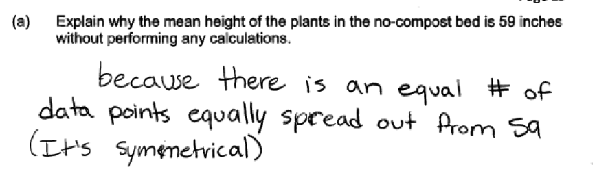
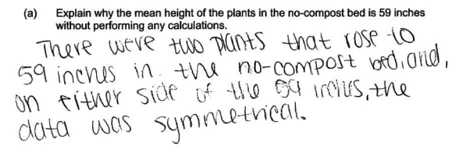 The following student response was also considered to be a correct response to part (a). Although the word symmetry is not mentioned, the student provides a correct verbal description of symmetry in the data distribution in terms of the deviations from the center.
Part (b)
There were several ways that students could show that the sum of the positive deviations from the mean and the sum of the negative deviations from the mean were equal for the compost data. Some students showed the actual calculation of the deviations, while others made use of the dot plots to illustrate the deviations graphically. This is illustrated by the following three student responses, which all provided correct responses to part (b). The first student response below also illustrates the balance point idea graphically, confirming understanding of the mean as a balance point of a data distribution.
Part (c)
In part (c) students were asked to give an interpretation of the MAD for the no-compost group. An ideal response to this part includes an interpretation of the MAD as the average or typical distance from the mean for the values in the no-compost data set. The following response illustrates this and was scored as essentially correct or part (c).
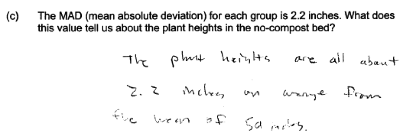 The following response also provides an interpretation of the MAD as an average distance from the mean. However, this response was scored as only partially correct for part (c) because it incorrectly uses the term variable instead of data value and the interpretation is not in context.
Part (d)
To demonstrate understanding of the concepts assessed in part (d) of this question, students needed to express the difference in means as a multiple of the MAD and then use that information to draw an informal inference about the difference in mean height for plants in beds with compost and plants in beds with no compost. Ideally they would compare the computed difference in means expressed as a multiple of the MAD to a benchmark value of 2, and then conclude that the difference in means is meaningful because the difference in means is greater than 2 MADs. The following two student responses were all scored as essentially correct because they include correct calculations, compare the difference in means expressed in terms of the MAD to a benchmark value and reach a correct conclusion.
 The following student response also indicates a solid understanding of the concepts assessed in part (d), but was scored as only partially correct because of the incomplete calculation in the first section of this part.
Common misunderstandings
Part (a) Understand the mean as a balance point
Responses that were not scored as essentially correct for part (a) generally either confused the mean with the median or the mode, or thought that the mean had to have an equal number of observations both above and below. The most common misconception was to confuse the mean and the mode of a data set. This is illustrated by the following two student responses that all indicate that 59 is the mean because there were more 59’s in the data set than there were for any other number.
Other students confused the mean and the median. Some indicated that the value of the mean has to be equal to the value of the median, which is not always the case. In this data set, the value of the mean and the value of the median happen to be equal because of the symmetry in the data distribution. The following two student responses illustrate this and were not considered correct for part (a) because they do not mention symmetry.
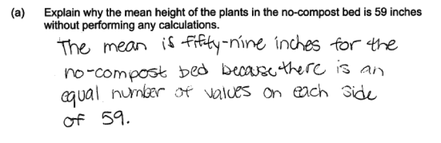
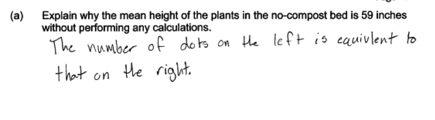
 Some students also confused the definition of the mean with the definition of the median. This confusion is demonstrated in the following two student responses where the students indicate that the mean is 59 because there are an equal number of observations above 59 and below 59.
Parts (b)
Verify that the mean is the point for which the sum of the positive deviations and the sum of the negative deviations are equal
Many students did not know how to start this problem and were not familiar with the idea of the mean as the point that balances the sum of positive deviations and the sum of negative deviations. As a result, many students did not provide an answer to part (b). For students who did attempt part (b) but who provided responses that were not considered to be essentially correct, most did not understand how to calculate deviations from the mean. For example, the following student response included a correct calculation of the mean for the compost group, but then divided the mean by 5 (half the sample size).
Part (c)
Interpret the mean absolute deviation (MAD) in context
There were three common errors made by students when answering part (c). It appears that many students were not familiar with the MAD and so were not able to provide a reasonable interpretation of the value of the MAD. For example, consider the following two student responses. Each of these responses interprets the MAD of 2.2 as the difference in means for the two groups and says it means that plants in the no-compost group are on average 2.2 inches shorter. These responses are incorrect for part (c).

 The following student response also illustrates an incorrect interpretation of the MAD. In this response, the student indicates that because the MADs for the two groups are equal, there is no difference in the growth for the compost and no-compost groups. This student may be confusing the MAD and the mean.
 A second common mistake was to say that a MAD of 2.2 inches indicated that there was not much variability in the heights for the no-compost group without actually interpreting the actual value of 2.2 as the mean distance from the mean for observations in the data set. This is illustrated by the following two student responses. The first response was scored as partially correct for part (c), while the second was scored as incorrect for part (c) because it also lacks context.

 The third common mistake probably is the result of not reading the question carefully. A number of students focused on the statement that the MAD was equal for the compost group and the no-compost groups and indicated that this meant that the variability was similar for the two groups. Unfortunately they didn’t answer the actual question posed, which asked for an interpretation of the value of the MAD for the no-compost group. This is illustrated in the following two student responses, which were scored as incorrect for part (c).
Part (d)
Informally assess the degree of overlap of two numerical data distributions with similar variability, measuring the difference in centers by expressing it as a multiple of a measure of variability
Use measures of center and variability to draw informal comparative inferences
Students found part (d) difficult to answer and did not understand how to make informal inferences about the difference between two groups based on considering the difference in means expressed as a multiple of a measure of variability. The two CCSS standards addressed in this part of this question are a challenge for both students and for teachers who have not previously had to develop this understanding.
In the first section of this part, many students were not able to express the difference in means (5 inches) as a multiple of the MAD (2.2 inches, and were not able to correctly compute the desired value of 5/22 = 2.27. The most common error for students who attempted to answer the second section of this part was to ignore the answer from the first section and to base the answer on the absolute difference between the means of 5 inches. This was common even for student who correctly calculated the difference in means as 2.27 MADs in the first section of this part.
The following two student responses illustrate this disconnect between the two questions posed in part (d). In each case, the answer given to the second question is unrelated to the answer provided to the first question.
 Some students were not able to provide a correct answer to section 1, but then used the value from section 1 and compared it to a benchmark value of 2 to answer the question posed in the second section. This is illustrated by the following two responses that were both considered to be partially correct for part (d).
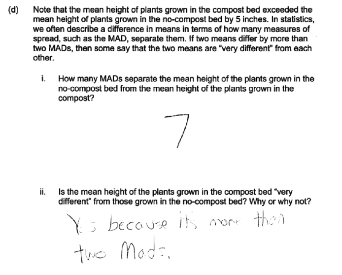 The student who provided the following response was on the right track in the first section, providing an indication that the student recognizes that 5” is greater than 2 MADs, but then doesn’t use this information in answering the second question.
The following student response was scored as only partially correct because the calculation in the first section was not quite correct and the communication in the response to the second section was considered to be weak.
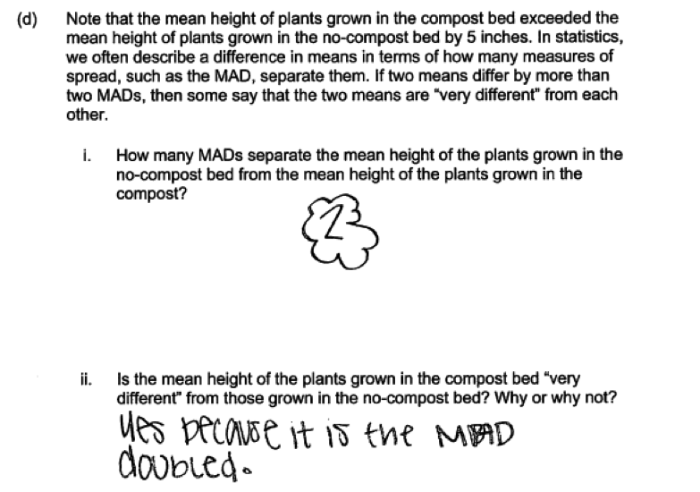
A few students answered part (d) incorrectly because they interpreted the fact that the MADs for the two groups were equal as meaning that there was no difference in the group means. This is illustrated by the following student response.
Resources
More information about the topics assessed in this question can be found in the following resources.
Free Resources
Common Core Progressions Documents
A discussion on informal comparative inference and of the intent of Common Core standards 7.SP.3 and 7.SP.4 and how this content might be developed in the classroom can be found in Common Core Tools progressions document for statistics in grades 6 – 8. See the discussion on pages 9 - 10.
Classroom and Assessment Tasks
Illustrative Mathematics has peer reviewed tasks that are indexed by Common Core Standard.
A task that involves interpreting the mean absolute deviation (MAD) is Math Homework Problems.
A task that involves drawing informal inferences about the differences between two groups is Offensive Linemen. The reasoning involved is similar to what is needed to answer parts (b) and (c) of this LOCUS question.
Guidelines for Assessment and Instruction in Statistics Education (GAISE)
Published by the American Statistical Association and available online, this document contains discussions of the mean as a balance point (pages 41 – 43) and the mean absolute deviation (page 44).
Resources from the American Statistical Association
Bridging the Gap Between Common Core State Standards and Teaching Statistics is a collection of investigations suitable for classroom use. This book contains an investigation that has students explore the mean as a fair share (“How expensive is Your Name?”, pages 85 – 97. See question 7 in particular). It also has an investigation that introduces deviations from the mean and develops the idea of the mean absolute deviation as a measure of variability (“How Long Are Our Shoes?”, pages 98 – 110).
Resources from the National Council of Teachers of Mathematics
The NCTM publication Developing Essential Understanding of Statistics in Grades 6 – 8 includes a section on measuring the amount of variability in a distribution on pages 24 – 27. This section includes a discussion of the mean absolute deviation. There is also a section on comparing distributions on pages 42 – 51.Although the focus of this discussion is on the median as a measure of center and the interquartile range as a measure of variability, there is an illustration of expressing a difference in centers as a multiple of a measure of variability (see page 50) that is particularly relevant to the content assessed in this LOCUS question.