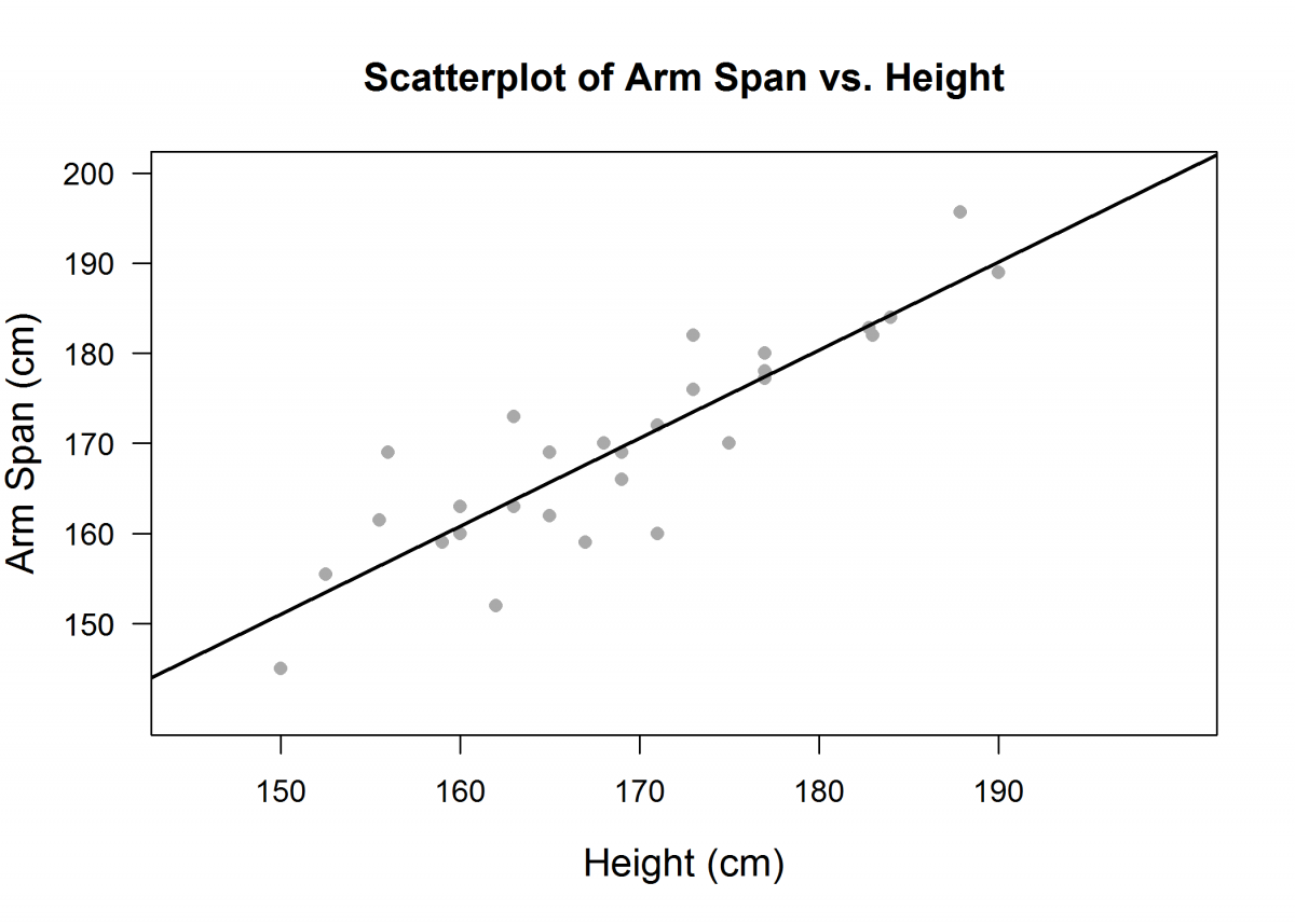
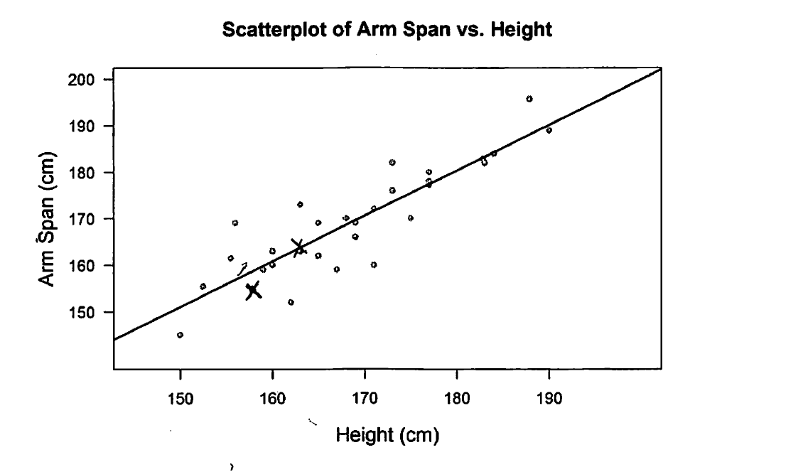
The heights (in centimeters) and arm spans (in centimeters) of 31 students were measured. The association between x (height) and y (arm span) is shown in the scatterplot below. The equation of the least-squares regression line for this association is also given.
estimated armspan = 4.5 + 0.977height
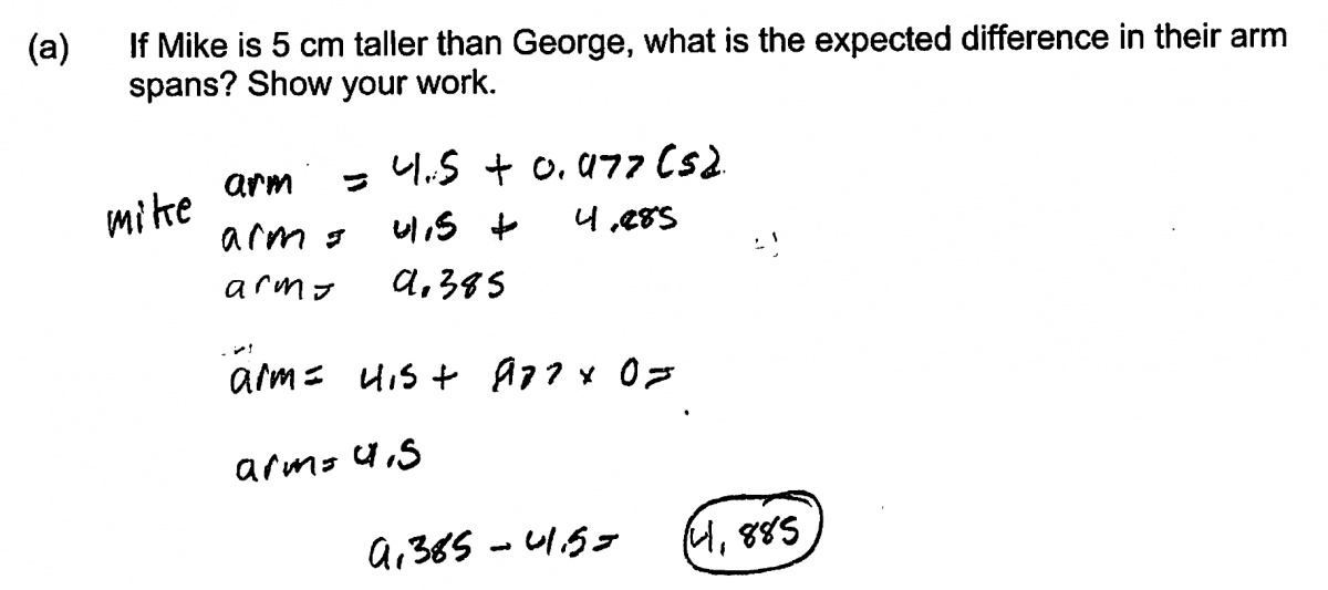
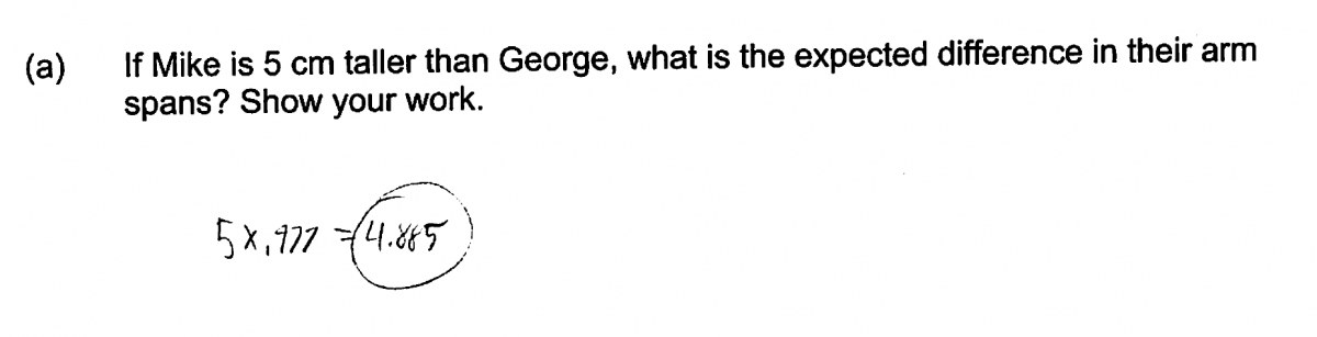
(a) If Mike is 5 cm taller than George, what is the expected difference in their arm spans? Show your work.
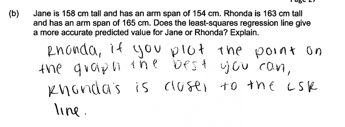
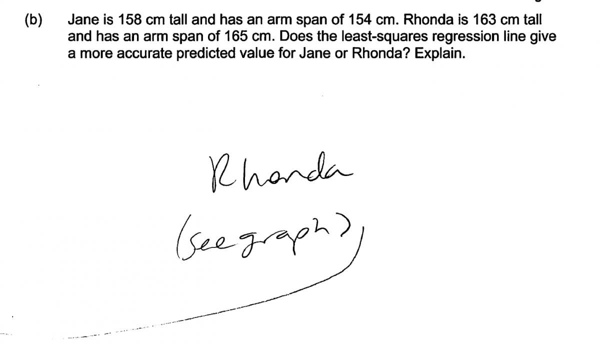
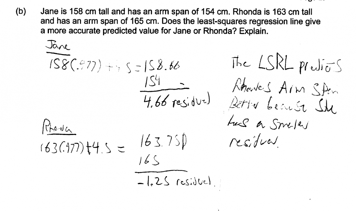
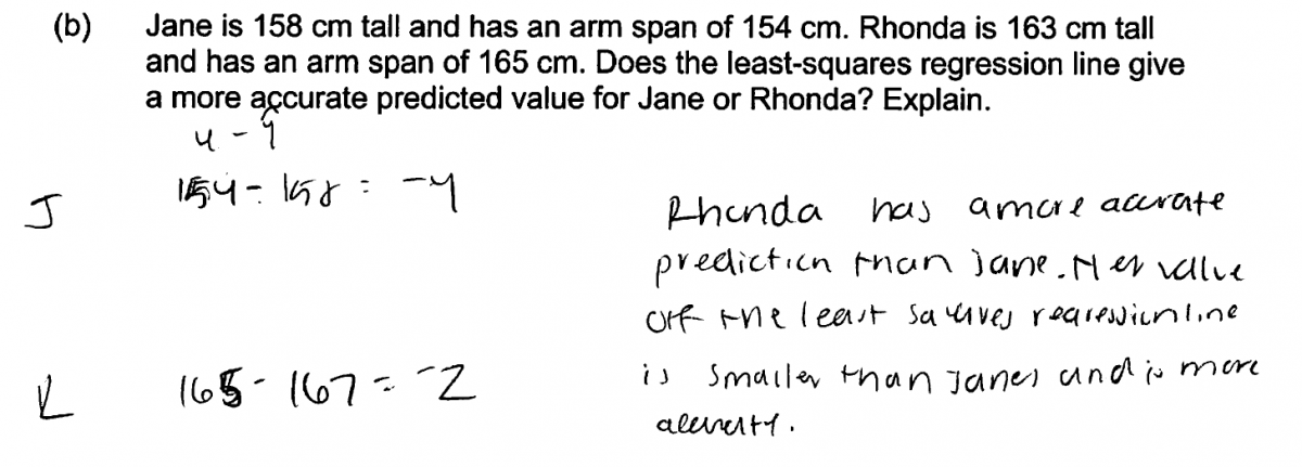
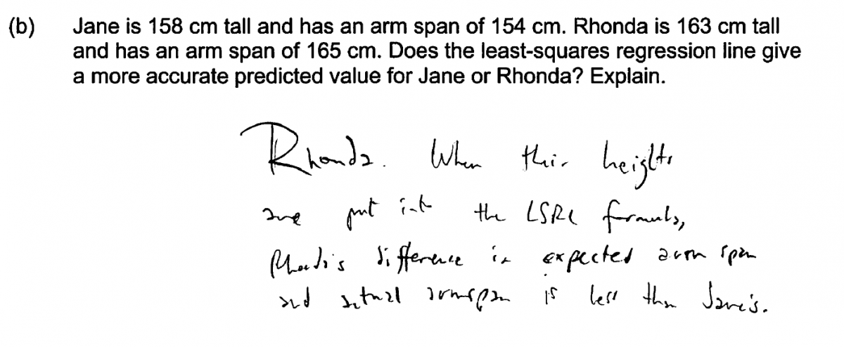
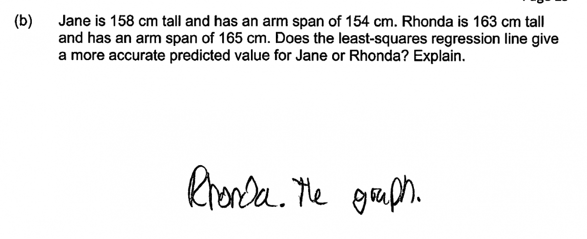
(b) Jane is 158 cm tall and has an arm span of 154 cm. Rhonda is 163 cm tall and has an arm span of 165 cm. Does the least-squares regression line give a more accurate predicted value for Jane or Rhonda? Explain.
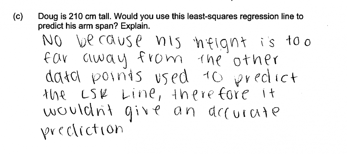
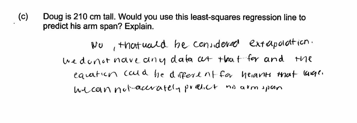
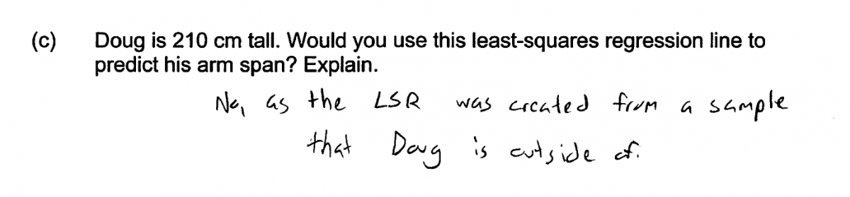
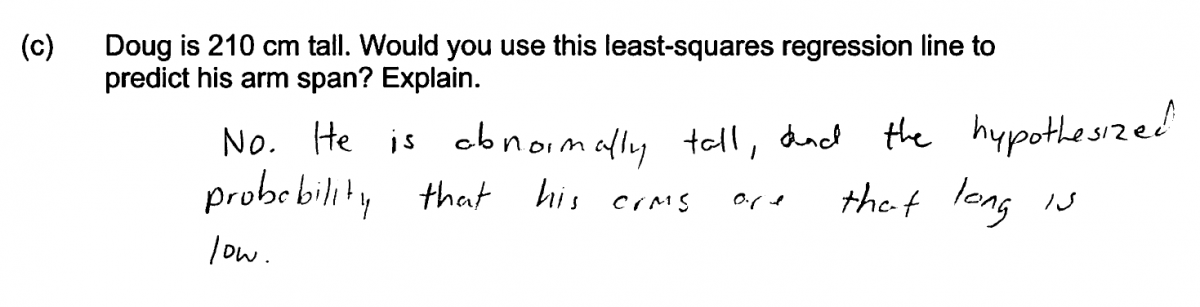
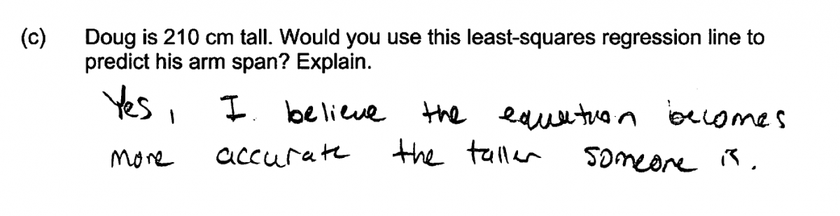
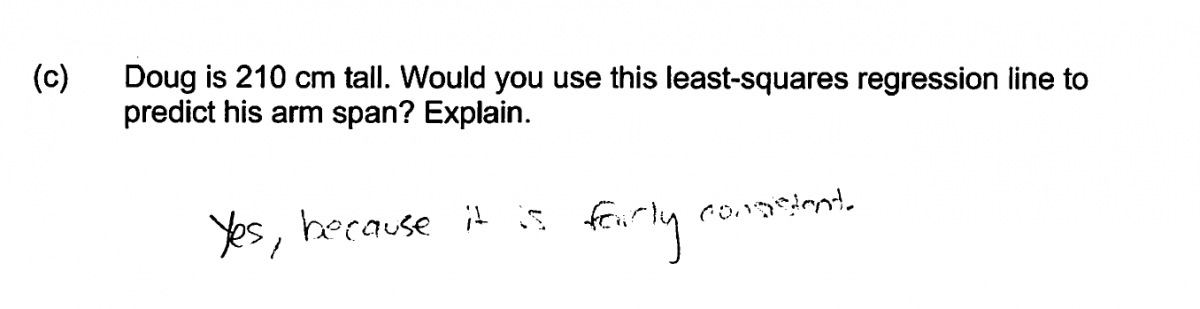
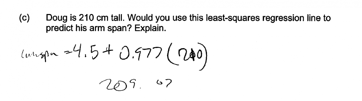
(c) Doug is 210 cm tall. Would you use this least-squares regression line to predict his arm span? Explain.
Overview of the question
This question is designed to assess the student’s ability to:
1. Recognize that the slope of the least-squares regression line represents the expected change in y associated with a 1 unit increase in x (part (a)).
2. Calculate a predicted value and the value of a residual given the equation of the least-squares regression line (part (b)).
3. Interpret a residual as the difference between an observed y value and the corresponding predicted y value (part (b)).
4. Recognize that the least-squares regression line should not be used to make predictions for x values that are far outside the range of the data used to determine the equation of the least-squares regression line (part (c)).
Standards
8.SP.3: Use the equation of a linear model to solve problems in the context of bivariate measurement data, interpreting the slope and intercept.
S-ID.6: Represent data on two quantitative variables on a scatter plot, and describe how the variables are related.
a. Fit a function to the data; use functions fitted to data to solve problems in the context of the data.
b. Informally assess the fit of a function by plotting and analyzing residuals.
c. Fit a linear function for a scatter plot that suggests a linear association.
S-ID.7: Interpret the slope (rate of change) and the intercept (constant term) of a linear model in the context of the data.
Ideal response and scoring
Part (a):
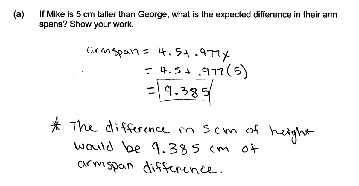
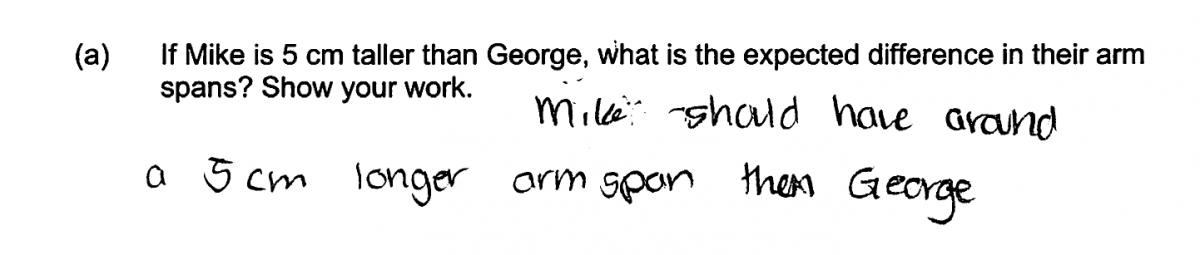
An ideal response to part (a) recognizes that the slope of the least-squares regression line can be interpreted as the expected change in arm span associated with a 1 cm increase in height. Students who understand this interpretation could then just multiply the given slope by 5 to obtain the expected difference in arm span for two people whose height differed by 5 cm. Responses that take this approach and that provide an explanation or include supporting work are scored as essentially correct for part (a).
While it was anticipated that students would take the approach described above in answering this question, the majority of students chose instead to assume heights for Mike and George with the height from Mike being 5 cm greater than the height for George. These heights were then used in the equation of the least-squares regression line to obtain predicted arm spans, and the difference in predicted arm spans was then calculated. While this approach is a lot more work, it leads to a correct answer, and responses using this method to obtain correct predicted values and the correct difference in predicted values are also scored as essentially correct for part (a).
Responses that used one of the two methods described but which included errors in the calculations needed to determine the expected difference were scored as partially correct for part (a).
Part (b):
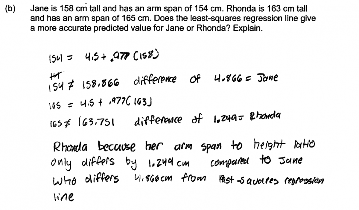
Part (b) asks students to determine which two predictions based on the least-squares regression line is more accurate. An ideal response to part (b) indicates that the prediction of Rhonda’s arm span is more accurate that the prediction of Jane’s arm span and provides justification for this choice. There are two ways that a student could provide a correct justification. One possible justification is based on calculating predicted values and residuals and then noting that the absolute value of the residual for Rhonda is less than the residual for Jane, indicating that the predicted arm span is closer to the actual arm span for Rhonda. Responses that provide a justification based on this method are considered to be essentially correct for part (b). Responses based on this method that include errors in calculating the predicted values or the residuals are considered to be partially correct for part (b).
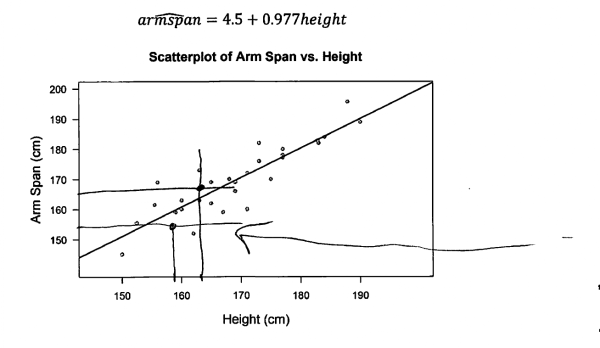
A second approach that could be used to support the choice of Rhonda in part (b) uses the given scatterplot and least squares line. Students using this method use the information on height and arm span for Rhonda and Jane to plot points on the scatterplot. They then note that the point that corresponded to Rhonda’s height and arm span is closer to the least-squares line than the point that corresponded to Jane’s height and arm span. Because predicted arm spans are points on the least-squares line, this means that the predicted arm span would be closer to the actual arm span for Rhonda. Responses based on this method are scored as essentially correct for part (b) provided that they include an explanation and show the two relevant points drawn on the scatterplot. Responses based on this method that include errors in plotting the points on the scatterplot are considered to be partially correct for part (b).
Part (c):
Part (c) asks students if it is reasonable to use the least-squares regression line to predict the arm span for Doug, an individual with a height of 210 cm. An ideal response to part (c) recognizes that 210 cm is quite a bit greater than the height of the tallest person in the group of 31 students that were used to develop the equation of the least-squares line. Because this represents an extrapolation beyond the range of the data, an essentially correct response to part (c) includes a statement that the least-squares regression line should not be used to predict Doug’s arm span.
Responses that indicate that it is not reasonable to use the equation of the least-squares regression line to predict Doug’s arm span but which do not specifically link this decision to Doug’s height being outside the range of the data used to develop the equation are considered to be only partially correct for part (c). Responses that do not include an explanation or that indicate that it is OK to use the least-squares regression line to predict Doug’s arm span are considered incorrect for part (c).
Sample responses indicating solid understanding
Part (a):
The following two student responses demonstrate understanding of the concepts assessed in part (a) of this question and both were scored as essentially correct for part (a). These responses illustrate two different approaches that could be taken in answering part (a). In the first response, the student assumes heights for Mike and George, calculates predicted heights and then calculates the difference in the predicted heights. In the second response, the student uses the slope of the given least-squares line to calculate the expected change in arm span associated with a five cm difference in height.
Part (b):
There are two ways that students could demonstrate an understanding of the concept assessed in part (b) of this question. One way is for the student to show that he or she understands that accuracy of a prediction based on the least-squares line is related to the distance of an observed point to the line. This would be done by plotting points representing (height, arm span) for Rhonda and for Jane on the given scatterplot and providing a justification based on comparing the distance of these two points to the line. This is illustrated by the following two student responses, which were scored as essentially correct for part (b).
The second apporach that a student could take is to demonstrate understanding that residuals provide information about the accuracy of predictions. For example, consider the following two student repsonses which received scores of essentially correct for part (b).
Part (c):
Responses that indicate an understanding of the concepts assessed in part (c) demonstrate an understanding of the danger in using a least-squares regression line to make predictions based on values that are far outside the range of the data used to determine the equation of the line. This is illustrated in the following student responses, which indicate that the line should not be used to predict Doug’s arm span and justify this based on the fact that Doug’s height is outside the range of height in the data set used to obtain the equation of the least-squares line.
Common misunderstandings
Part (a): Recognize that the slope of the least-squares regression line represents the expected change in y associated with a 1 unit increase in x.
Students generally did a reasonable job in responding to part (a) of this question, although not very many answered the question using the anticipated approach based on recognizing how the slope of the least-squares line could be used to answer this question. As a result, most students spent time calculating predicted values and finding the difference in order to answer this question.
The most common error in answering this question was made by students who realized that they needed to use the given equation of the least-squares line in some way, but did not use it appropriately. These students substituted 5 into the equation to obtain the predicted arm span for a person whose height was 5 cm! This is illustrated by the student responses below, which were scored as incorrect for part (a).
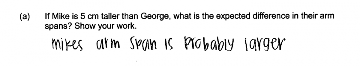
A few students did not know how to use the least-squares line to answer part (a). For example, consider the student response below. While this student has recognized that there is a positive relationship between height and arm span, the student was not able to provide a value for the expected difference, and this response was scored as incorrect for part (a).
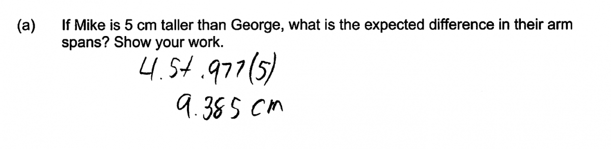
Finally, even though the question specifically asks students to show their work, some responses did not show supporting work and were scored as only partially correct. The student response below would have been considered correct (assuming that the student rounded to the nearest cm) if supporting work had been included.
Part (b): Calculate a predicted value and the value of a residual given the equation of the least-squares regression line. Interpret a residual as the difference between an observed y value and the corresponding predicted y value.
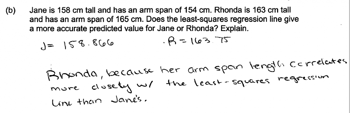
Students had more difficulty responding to part (b) than the other parts of this problem and there were a number of relatively common student errors. For example, some students calculated predicted values, but did not calculate residuals or explicitly compare the predicted values with the given actual arm spans for Rhonda or Jane. This is illustrated in the following student response, which received a score of partially correct for part (b) because it is not clear what the student means by the statement that “her arm span length correlates more closely with the least-squares regression line.”
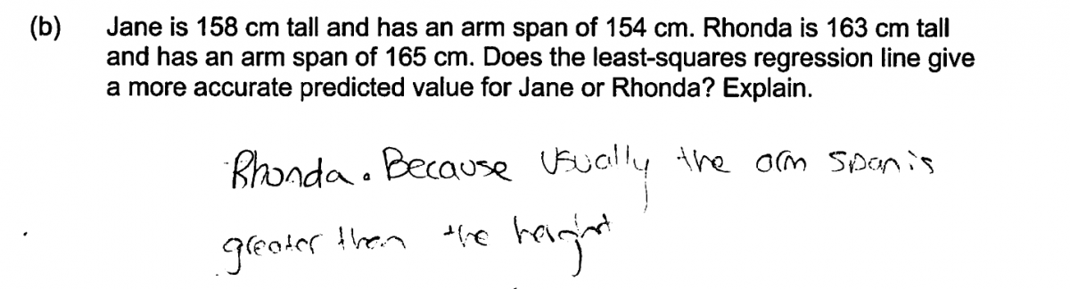
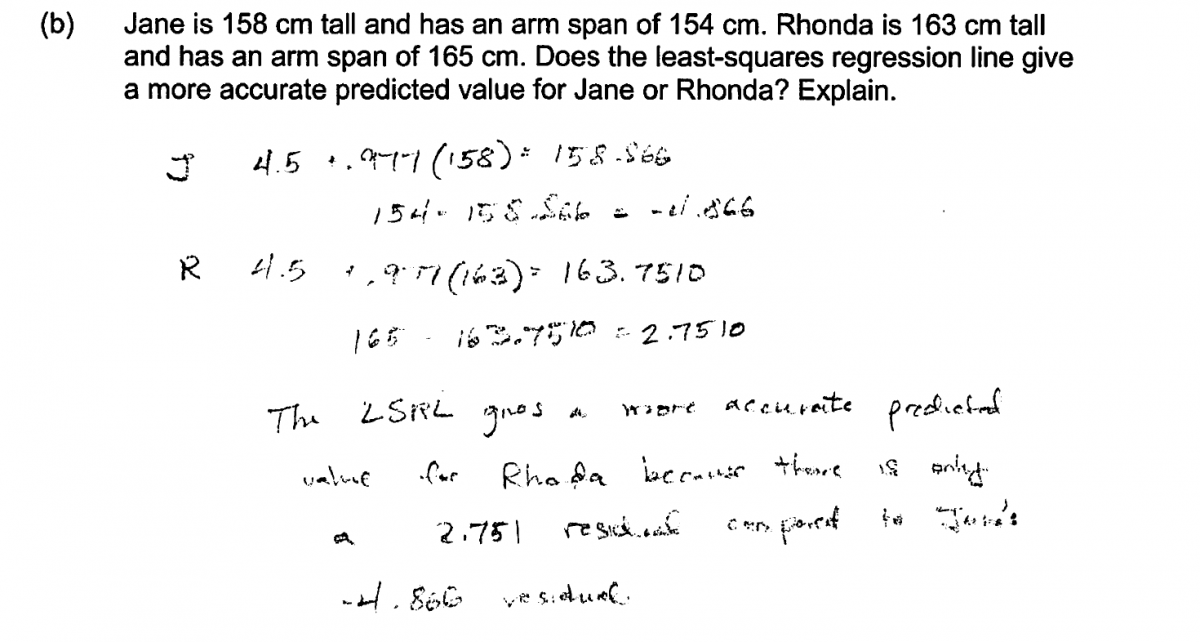
Many students correctly indicated that the prediction of Rhonda’s arm span was more accurate, but then provided an incorrect explanation. This error is illustrated in the following two student responses. In the first of these responses, the student calculates the residuals correctly but then provides an incorrect interpretation of those residuals. In the second response below, the provided justification does not include an explanation based on residuals or the distance of the points to the line. While it is true that the scatterplot and least-squares line indicate that arm span tends to be greater than height, this alone is not enough to guarantee that predictions would be more accurate for someone whose arm span is greater than his or her height. Each of these responses was scored as partially correct for part (b).

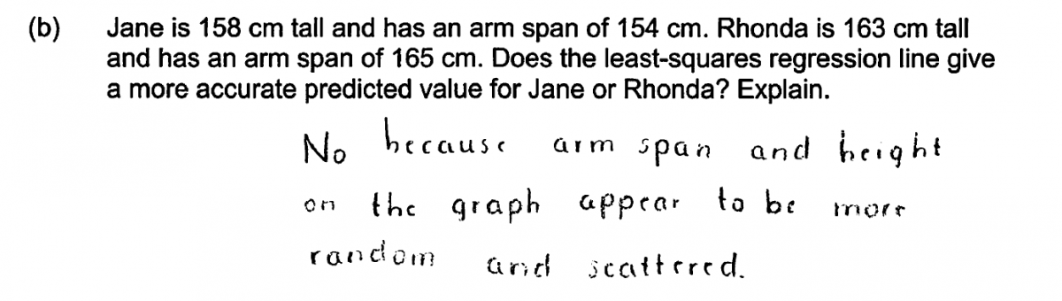
Some student responses indicated that they believed that it is not possible to tell which prediction would be more accurate. For example, consider the student response below. In this response, the student indicates that the line would not be more accurate for one or the other because there is a lot of scatter around the regression line. While that does imply that some prediction errors might be large, it is still possible to evaluate the arm span predictions for Rhonda and Jane and to determine which is closer to actual arm span.
It was also common for students to make errors in calculating the predicted values or the residuals. The following two student responses are typical of the responses of students making this error. Each of these responses were scored as partially correct for part (b).
Finally, some students provided an explanation that was found to be insufficient for a score of essentially correct for part (b). In the first of the two student responses below, the student explains how it would be possible to arrive at an answer, but gives no evidence that the steps described were actually carried out. This response was scored as partially correct for part (b). The second of the two responses below was scored as incorrect for part (b). Although it references the graph, there were no markings on the graph to indicate that the student has plotted the two relevant points and considered the distance of these points to the least-squares regression line.
Part (c): Recognize that the least-squares regression line should not be used to make predictions for x values that are far outside the range of the data used to determine the equation of the least-squares regression line.
Responses to part (c) that were not scored as essentially correct generally made one of two common errors. Some students correctly indicated that the least-squares regression line should not be used to make a prediction of Doug’s arm span, but did not provide an explanation that clearly indicated that the reason a prediction should not be made was that Doug’s height was outside the range of height in the data set used to determine the equation of the least-squares line. For example, in the student response below, the student notes that Doug is “abnormally tall” but does not compare Doug’s height to the heights in the data set. For this reason, this student response was scored as only partially correct for part (c).
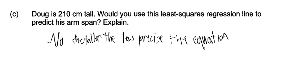
The response below also indicated that the least-squares line should not be used to make a prediction, but justifies this by saying the equation is less precise for tall people. While this might be true, there is nothing in the given scatterplot to suggest that this is the case and it does not address the key issue of extrapolation beyond the range of the data. This response was also scored as only partially correct for part (c).
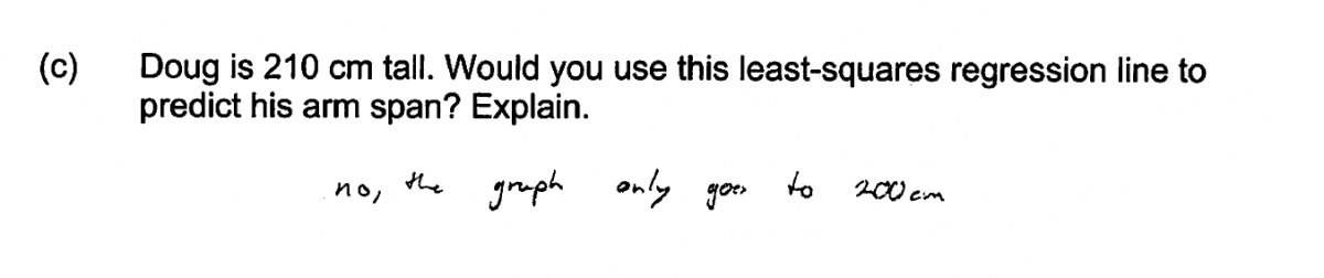
The following student responses were also scored as partially correct for part (c). Although they appear to be on the right track, it is not clear that they are looking at the actual range of values in the data set or just the scale on the axis. Because it is not clear that these students are addressing the issue of extrapolation beyond the range of the data, these responses were not scored as essentially correct.
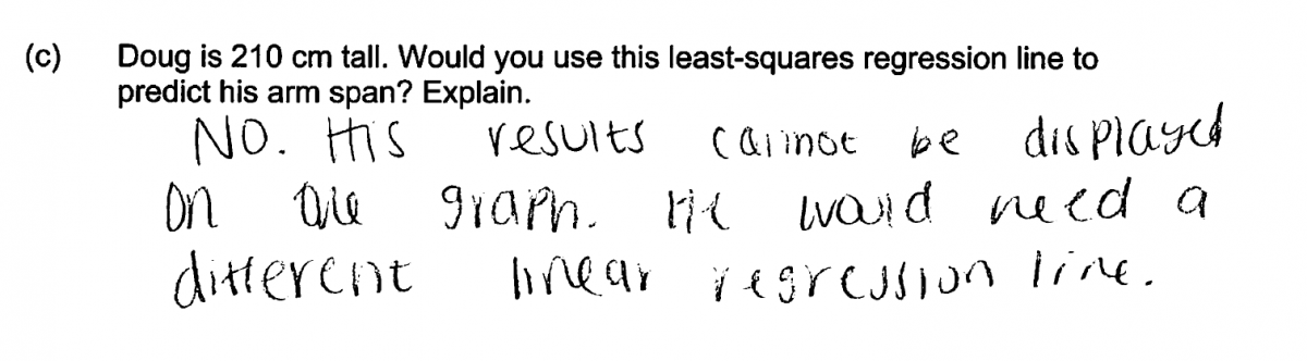
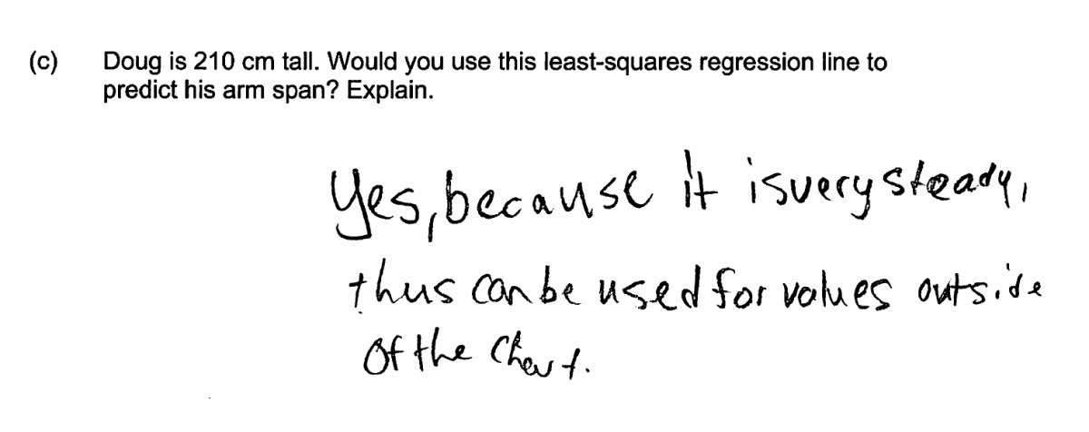
The second common student error was made by students who did not recognize that the question was asking for a prediction for a height value that was far outside the range of the data set. Students making this error generally indicated that it was appropriate to use the least-squares line to make a prediction of Doug’s arm span. The four responses below all make this error. Some also include incorrect statements in the explanation. For example, the second response below states that the least-squares line “can be used for values outside of the chart.” These four responses were all scored as incorrect for part (c).

Some students didn’t actually answer the question asked, and instead just used the equation of the least-squares line to predict Doug’s arm span. This error is illustrated by the following student response, which was also scored as incorrect for part (c).
Resources
Resources
More information about the topics assessed in this question can be found in the following resources.
Free Resources
Lessons
Statistics Education on the Web (STEW) has peer reviewed lessons plans. Three lessons related to the topics assessed in this Locus question are:
Scatter It! (Predict Billy’s Height)
Classroom and Assessment Tasks
Illustrative Mathematics has peer reviewed tasks that are indexed by Common Core Standard.
A task that develops content related to parts (a) and (c) of this Locus question is:
A task that explores residuals and is relevant to the content of part (b) of this Locus question is:
Restaurant Bill and Party Size
Three tasks that include the interpretation of slope in context and that are relevant to the content assessed in part (a) of this Locus question are:
Guidelines for Assessment and Instruction in Statistics Education (GAISE)
Published by the American Statistical Association and available online, this document contains an example similar to this Locus question (Linear Regression Analysis—Height vs. Forearm Length) on pages 80 – 82.
Resources from the American Statistical Association
Bridging the Gap Between Common Core State Standards and Teaching Statistics is a collection of investigations suitable for classroom use. This book contains a section on exploring relationships (Section 5). Investigation 5.3 in this section develops the skills assessed in part (a) of this question.
Resources from the National Council of Teachers of Mathematics
The NCTM publication Developing Essential Understanding of Statistics in Grades 6 – 8 includes a section on summarizing linear trends on pages 62 – 66.