Stella saw the following headline in a national newspaper: “30 Percent of High School Students Favor Extended School Day.” She wondered if the percentage of students at her school who favor an extended school day was less than 30 percent. To investigate, she selected a random sample of 50 students from the 1,200 students at her school and asked each student in the sample if he or she favors an extended school day.
Only 12 of the students in the sample favored an extended school day. Because the sample percentage is (12/50)100 = 24%, Stella thinks that fewer than 30 percent of the students at her school favor an extended school day. She wonders if it would be surprising to see a sample percentage of 24 or less if the school percentage is
really 30.
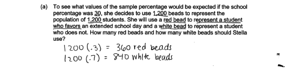
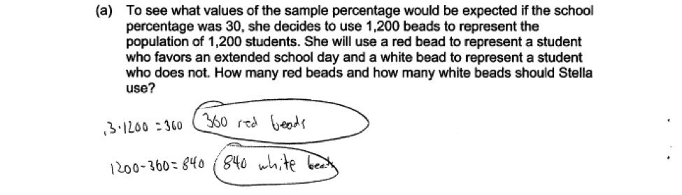
(a) To see what values of the sample percentage would be expected if the school percentage was 30, she decides to use 1,200 beads to represent the population of 1,200 students. She will use a red bead to represent a student who favors an extended school day and a white bead to represent a student who does not. How many red beads and how many white beads should Stella use?
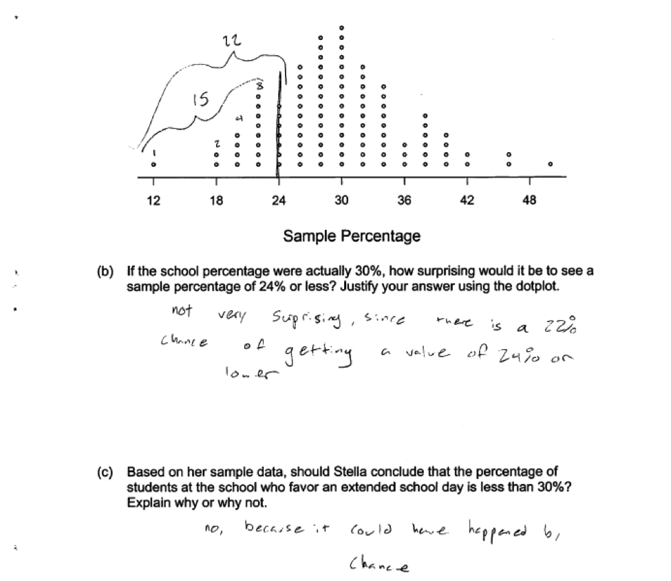
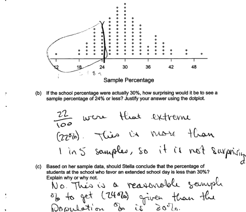
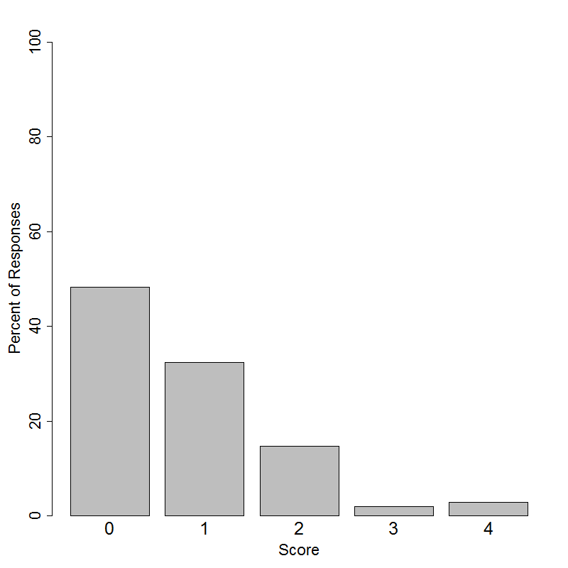
Stella put all the beads in a box. After mixing the beads, she selected 50 of them and computed the percentage of red beads. She put the 50 beads back in the box and repeated this process 99 more times. Then, she made the following dotplot of the 100 sample percentages:
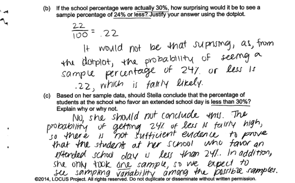
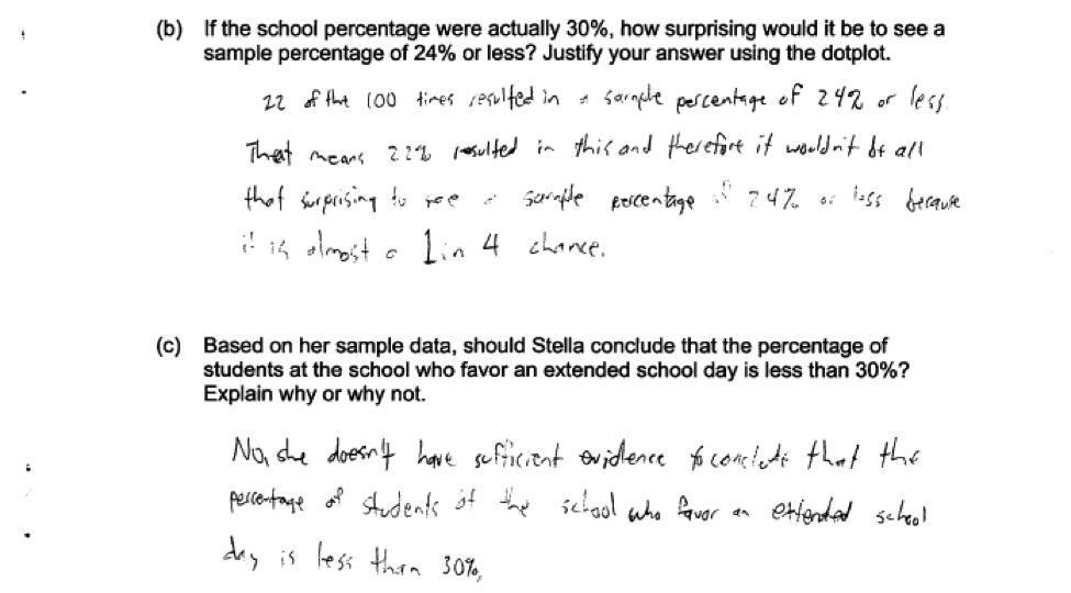
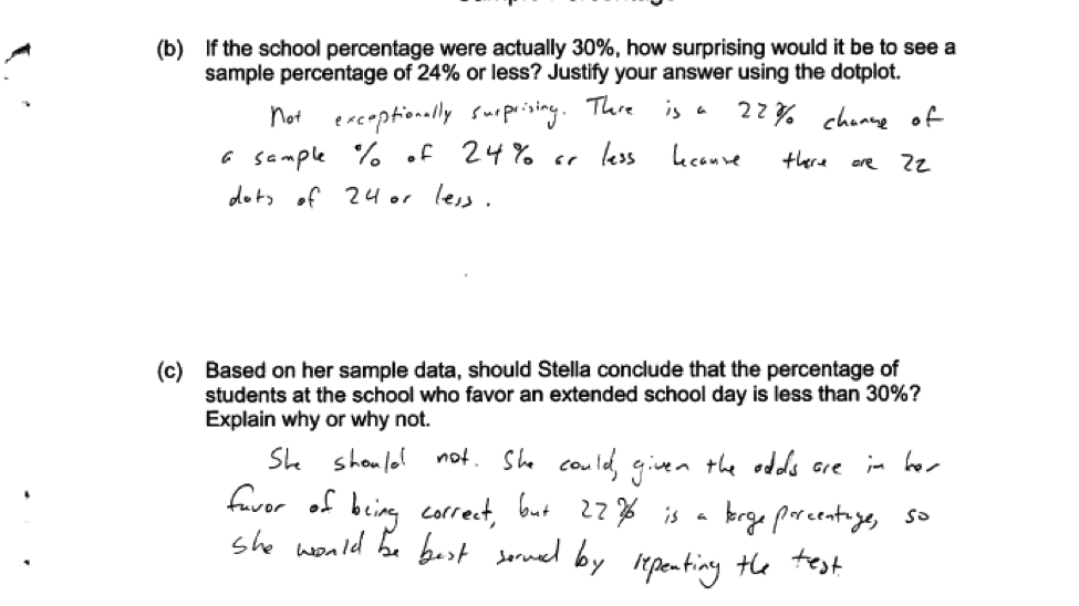
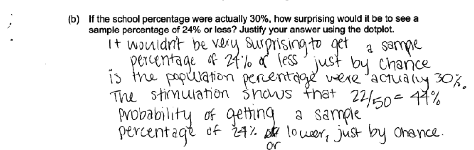
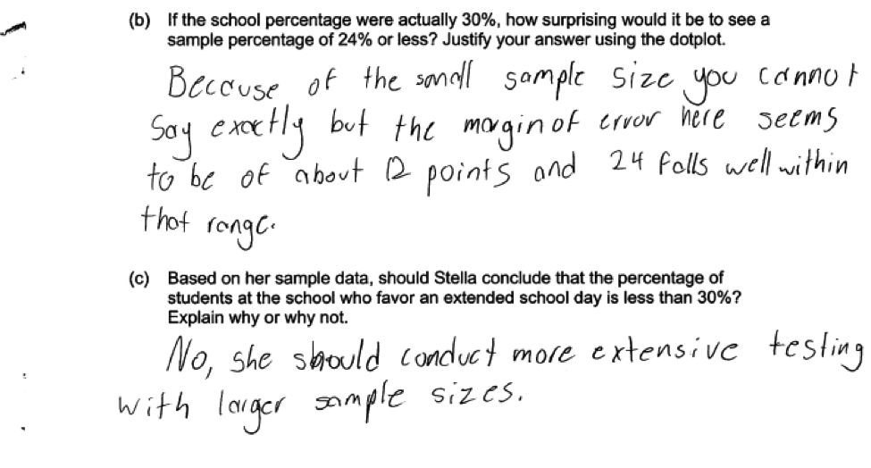
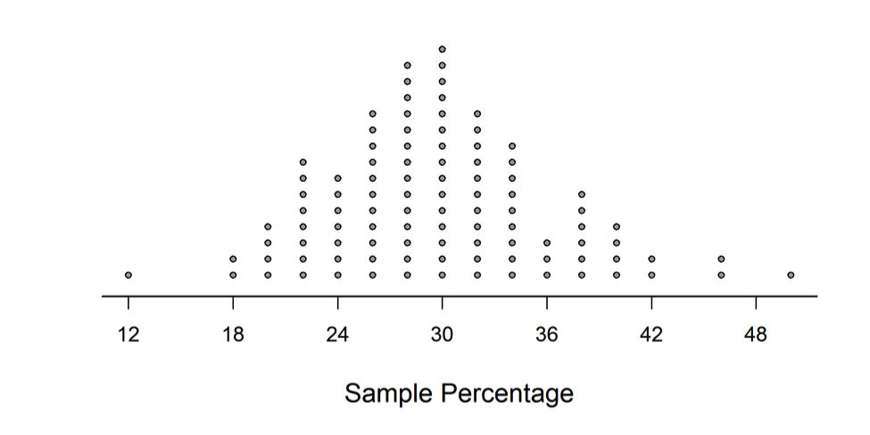 (b) If the school percentage were actually 30%, how surprising would it be to see a sample percentage of 24% or less? Justify your answer using the dotplot.
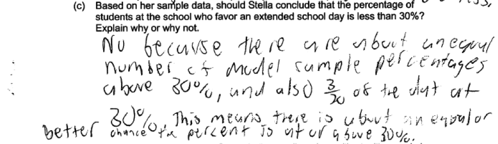
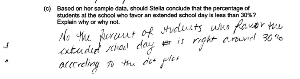
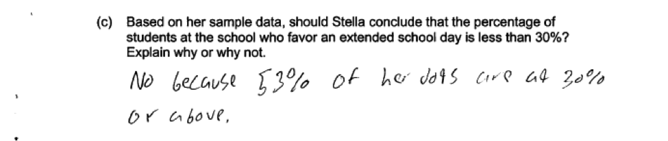
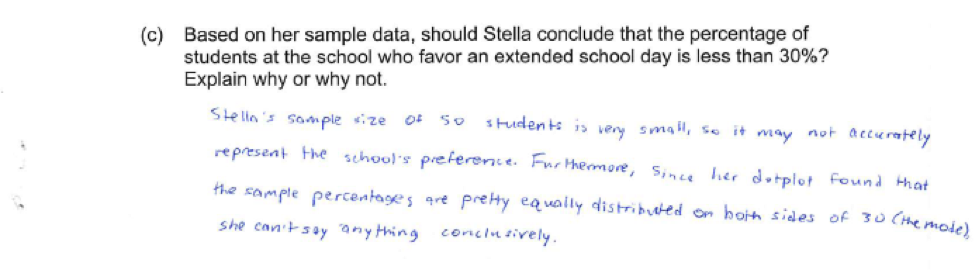
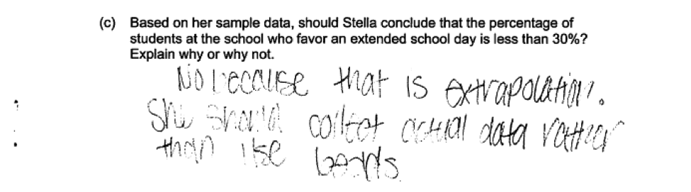
(c) Based on her sample data, should Stella conclude that the percentage of students at the school who favor an extended school day is less than 30%? Explain why or why not.
Overview of the question
This question is designed to assess the student’s ability to:
1. Develop a model that could be used to carry out a simulation (part (a)).
2. Use a simulated sampling distribution to decide if an observed sample percentage is one that is likely to be observed by chance given a particular hypothesized population percentage (part (b)).
3. Use a simulated sampling distribution to draw a conclusion about a population in a way that takes sampling variability into account (part (c)).
Ideal response and scoring
Part (a):
An ideal response to part (a) recognizes that an appropriate model for the population of interest (30% favoring an extended school day) that uses 1,200 beads to represent the 1,200 students at the school would need to include 30% red beads and correctly calculates that this means there should be 360 red beads and 840 white beads. If one of these two values is calculated incorrectly, the response is considered partially correct.
Part (b):
An ideal response to part (b) notes that a sample percentage of 30% would not be surprising for a sample of size 50 from a population in which 30% favored an extended school day and provides a correct justification based on the given simulated sampling distribution. A response that does this and makes it clear that the reasoning is based on using a boundary of 24% (the observed sample percentage) is considered essentially correct. Although not required, if the response uses the simulated sampling distribution to approximate and interpret a p-value, the calculation and interpretation must be correct. If the interpretation is incorrect, the response is considered only partially correct.
A response that correctly indicates that a sample percentage of 24% would not be surprising, but does not clearly link the justification to the given simulated sampling distribution is also considered partially correct. A response in which the justification is incorrect or missing is considered incorrect.
Part (c):
Part (c) asks if it is appropriate to conclude that the population percentage is less than 30% based on a sample percentage of 24%. An ideal response to part (c) indicates that the difference between the observed sample percentage of 24% and the hypothesized percentage of 30% is not statistically significant or that it could be explained by sampling variability alone. In order to be considered essentially correct, the response also needs to provide a justification that is consistent with the response in part (b).
A response that indicates that the difference is not statistically significant but provides an explanation that does not indicate how the decision was made or that is not in context is considered partially correct.
A response that indicates that it is reasonable to conclude that the population percentage is less than 30% may be considered partially correct if it is consistent with an incorrect answer given in part (b). If this is not the case, then such a response is considered incorrect. A response to part (c) in which the explanation is missing is also considered incorrect.
Sample responses indicating solid understanding
Part (a) of this question was included to help students understand the simulation described in the lead in to parts (b) and (c). Most students had little difficulty with part (a). In reading the responses to parts (b) and (c), these two parts were read and scored together because it was often the case that what was written in part (c) completed a partial answer in part (b) or a partial answer in part (c) is completed by the explanation given in part (b).
The following student response shows a good understanding of the concepts assessed by this question and received a score of 4. The number of red beads and the number of white beads is correctly calculated in part (a). In part (b) the response indicates that a sample percentage of 24% would not be surprising and clearly links the explanation to the given simulated sampling distribution. The response in part (c) correctly concludes that it is not reasonable to conclude that the population percentage is less than 30% based on the sample data, and while the response would have been stronger if the term “prove” had not been used, part (c) was still scored as essentially correct. With all three parts essentially correct, this student response received a score of 4.
 The following student response also received a score of 4, and illustrates the need to read parts (b) and (c) together. Part (c) by itself is not complete, but the necessary explanation is given in part (b).
 There are a number of ways that a student could demonstrate understanding of the concepts assessed in parts (b) and (c). For example, the following responses were also scored as essentially correct for both parts (b) and (c) (read and scored together):
 The following response was scored as partially correct for part (b) because the explanation does not provide a clear link to the given simulated sampling distribution. The question specifically asks for an explanation in terms of the dotplot.
 Another example of a response to part (b) that shows understanding of the underlying concepts but which was considered only partially correct is shown below. In this response, the p-value is computed incorrectly.
Common misunderstandings
Part (a) Develop a model that could be used to carry out a simulation
Most students had little difficulty with part (a). Responses that were not considered essentially correct on part (a) generally made one of two errors. Some calculated only the required number of red beads and did not give the number of white beads. Others used the observed sample percentage of 24% to determine the number of red beads rather than the hypothesized percentage of 30%. It is important that students read the question carefully and provide all of the information requested in the question (here, both the number of red beads and the number of white beads).
Parts (b) and (c) Use a simulated sampling distribution to decide if an observed sample percentage is one that is likely to be observed by chance given a particular hypothesized population percentage and use a simulated sampling distribution to draw a conclusion about a population in a way that takes sampling variability into account.
The most common student error in parts (b) and (c) was to failure to understand that the simulated sampling distribution represents what might be expected IF the population percentage were 30%. Many student responses indicated that they believed that the given distribution was what would happen when sampling from the actual populations and gave an argument based on 30 being at the center of the distribution. Surprisingly, this sometimes occurred in part (c) even after the student had interpreted the simulated sampling distribution correctly in answering part (b). This error in thinking is illustrated in the following student responses.
 Another student error resulting from failure to understand the simulated sampling distribution is illustrated in the following response. In this response, it is clear that the student does not understand that the dots in the dotplot represent a percentage based on a sample of 50 students from a population in which 30% of the students favor an extended school day and that the student is interpreting the dots in the dotpot as somehow representing individual students.
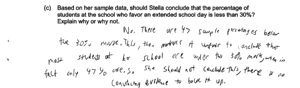 Some student responses demonstrated that the student did not really understand the concept of sampling variability, indicating that it would be reasonable to conclude that the population percentage was less than 30% because most of the dots in the dotplot of the simulated sampling distribution represented values that were 30 or less. This is illustrated in the following responses.

 Another common mistake was to focus on the sample size. Even thought the sample size was 50, many responses indicated that no conclusion could be drawn because the sample size was too small. This is illustrated in the following responses.
 Finally, some students did not understand the purpose of simulation in this context, as illustrated in the following response.
Student performance
Resources
An understanding of sampling variability is critical to the development of students’ statistical reasoning.
More information about this topic can be found in the following resources.
Free Resources
Lessons
Statistics Education on the Web (STEW) has peer reviewed lessons plans that can be found at http://www.amstat.org/education/stew/index.cfm. Some lessons related to the topic of this question are
Population Parameters and M&M’s
What Percent of the Continental US is within One Mile of a Road
Using Dice to Introduce Sampling Distributions
Applets
There are a number of online applets that can be used to illustrate simulated sampling distributions. One easy to use applet that is worth checking out is part of the RossmanChance applet collection.
Classroom and Assessment Tasks
Illustrative Mathematics has peer reviewed tasks that are indexed by Common Core Standard. Standard S.IC.4 is relevant to the concept of sampling variability in a sample proportion. One tasks relevant to this standard is
Guidelines for Assessment and Instruction in Statistics Education (GAISE)
Published by the American statistical Association and freely available online, this document contains a discussion sampling variability for a sample proportion on pages 67 – 69.
Common Core Progressions Documents
A discussion of the intent of Common Core standard S.IC.4 and how this content might be developed in the classroom can be found in Common Core Tools progressions document for statistics in grades 9 – 12. See the discussion on pages 8 - 12.
Resources from the American Statistical Association
Making Sense of Statistical Studies is a collection of investigations suitable for classroom use. Section IV looks at drawing conclusions from data and is relevant to the concepts assessed in this question. Investigation 13 (The Internet—Information or Social Highway) and Investigation 14 (Evaluating the MySpace Claim) are activities suitable for classroom use that explore concepts assessed in this question.
Resources from the National Council of Teachers of Mathematics
The NCTM publication Developing Essential Understanding of Statistics in Grades 6 – 8 includes a section on the big idea “Samples and Populations.” See the discussion on pages 67 – 78.
The NCTM publication Developing Essential Understanding of Statistics in Grades 9 – 12 includes a section on the big idea “Describing Variability.” The discussion on pages 32 – 43 is relevant to the concepts assessed in this question.
The NCTM publication Navigating through Data Analysis in Grades 9 – 12 includes a chapter titled “Making Decision with Categorical Data” that is related to the concepts assessed in this question.